|
|
|
Let us recall the wave equation we proved in the last page.
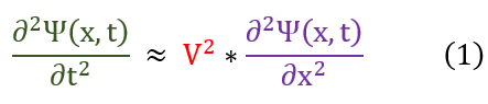
Now let us tackle the solution to this differential equation. To do this, let us analyze both sides of this equation:
RHS: T and P_L were constants and hence so is the wave velocity. For a non-varying x, the RHS is a constant.
LHS: For a non-varying x, the LHS does not have to be a constant (depends on t).
One may ask: HOW IS THIS POSSIBLE? This equation must always be true! If one side is constant, then by default both have to be. Therefore, to resolve this dispute, both sides must always constant. If I do not move my x position, and time keeps running, I do not change either side of the equation. If I freeze time, and compare x positions, I still cannot change either second derivative. The time and position coordinates are not dependent on each other. We call this a standing wave.
For standing waves, time and position are independent of each other and hence we can use a technique called separation of variables where psi(x,t) = psi(x)*psi(t).
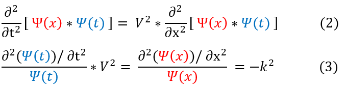
In order to make sure everyone is following, let us review some key steps below:
2 to 3: Since psi(x) is a constant in the d/dt derivative, it can just be divided out. Similarly for the psi(t) in the d/dx
derivative. Equation 2 and 3 are equal to a constant. I arbitrarily called the constant in equation 3 '-k^2'.
One might wonder why I named the constant -k^2. It was completely arbitrary. Some familiar with differential equations may recognize that this makes the differential equation like a sinusoidal function, but, if not, just note that I really could have arbitrarily called the constant anything.
It can also be appreciated that -k^2 must be a negative number. If k was imaginary, and -k^2 was positive, the solution to the differential equation would be an exponential function. However, as the string does not diverge off into infinity, but rather oscillates around the origin, it can be appreciated that k must be a real number.
Another note about the constant is that it does have significant meaning. As you might guess, the fact that both sides of this equation equals the same constant is little of a coincidence. It was determined experimentally to be the wavevector of the standing wave. k = 2*pi/(wavelength). It carries a page-load of meaning, one of the most significant is the wave propagation direction. However, for quantum mechanics at this stage, it is little more than a constant = 2*pi/(wavelength)
It is time to solve each differential equation separately.
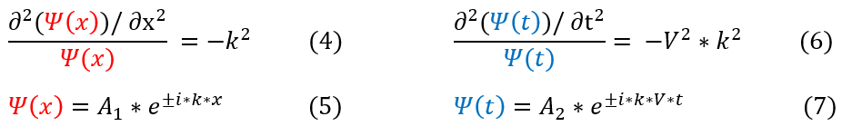
In order to make sure everyone is following, let us review some key steps below:
4 to 5: Solution to the second order differential equation where A_1 is some arbitrary constant.
6 to 7: Solution to the second order differential equation where A_2 is some arbitrary constant.
One may note that k and V are both constants quantities about the wave. Analyzing the physical meaning of each constant we can see that k*V = omega = w = angular frequency of the oscillations.

Now it is time to combine the two equations we have into one to get the full solution to the first approximation of the wave equation.

The equation above represents the full solution to any wave equation in 2-D. Where 'A' is some arbitrary constant. While, this is the most general form, it can be found graphically that kx-wt would yield a wave moving in the positive x-direction. This positive x-direction will be the arbitrary direction chosen to deal with for this type of wave. One can additionally note that extending a wave on a string into the y dimension would yield what is called a plane wave.
|
|
|
