We have generally solved the Bound State (finite square well) problem in the last page. While the next step is to quantitatively solve the problem, let us first qualitatively predict what the wave function should look like. For a reminder, the pictorial representation of the problem is described below:

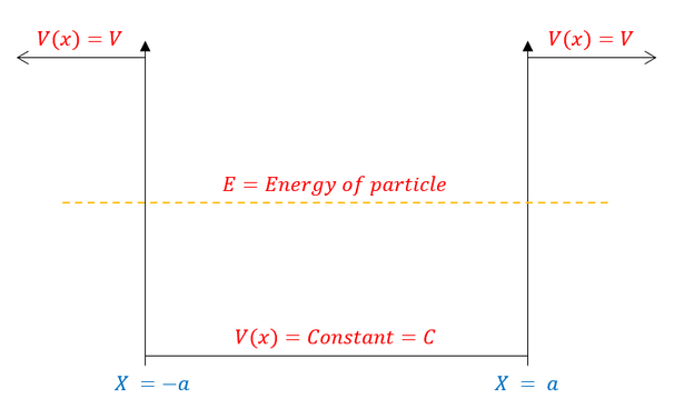
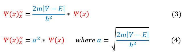
          For the region inside the box, we found the equations below: (see the mathematical setup page for the derivation):

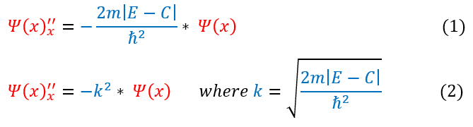
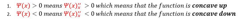
          From just observing equation 2 above: one can notice that no matter what ‘k’ equals, it is always a positive number (as we define 'k' to be real). Therefore, whether the second derivative is either positive or negative is completely dependent on whether the wave function is positive or negative. We can analyze these two cases below:

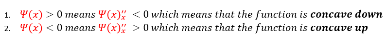
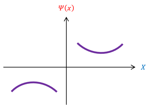
          Basic algebra tells us that a negative second derivative is a concave down function and a positive second derivative is a concave up function. Hence, the function is concave down above the x axis (when psi(x) is positive) and concave up below the x axis (when psi(x) is negative). We call this type of analysis the shooting method. We can pictorially represent this below:

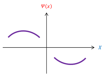
          Notice that the function always points towards the x axis, similar to oscillatory functions (which validates the sin and cosine functions found on the previous page). This is fine because our criteria for usable wave functions is for them to be normalizable and eventually decay to zero (the x axis) at +/- infinity, which is possible in this situation. The only quality used to generate these sinusoidal functions was that the energy was greater than the potential.

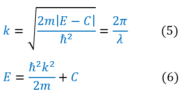
          Now let us qualitatively sketch the classically forbidden region. Let us first recall the mathematical equations we derived in the last page:

          From just observing equation 4 above: one can notice that no matter what ‘α’ equals, it is always a positive number (as we define 'α' to be real). Therefore, whether the second derivative is either positive or negative is completely dependent on whether the wave function is positive or negative. We can analyze these two cases below:

          Basic algebra tells us that a negative second derivative is a concave down function and a positive second derivative is a concave up function. Hence, the function is concave up above the x axis (when psi(x) is positive) and concave down  below the x axis (when psi(x) is negative). We can pictorially represent this below:

          Notice that the function always points away from the x axis. This is problematic because our criteria for usable wave functions is for them to be normalizable and eventually decay to zero (the x axis) at +/- infinity, which is not always possible in this situation. This leaves us with a constraint: the wave function must exponentially decay to the axis, without deviating, at the ends of the wave function. Basically, instead of dipping and coming back up, we must have the wave function only dip. The only quality used to generate these functions was that the energy was less than the potential.

          While this constraint may seem harmless, it actually has very dramatic implications. To understand these implications, let us analyze the energy of the particle. Energy is a function of 'k' and 'α.' Let us look at the 'k' definition:

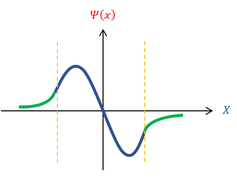
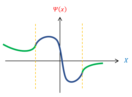
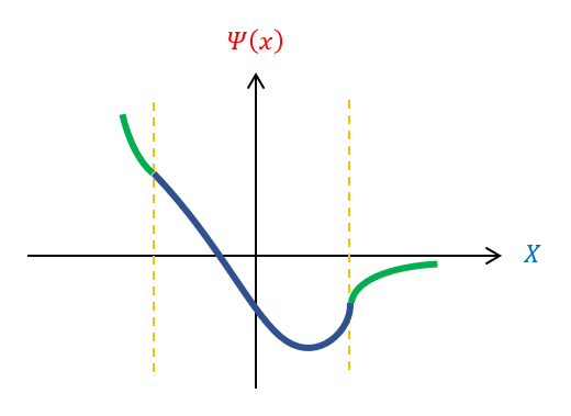
           All the variables in equation 6 (besides ‘k’) is a constant. Hence, if ‘k’ is continuous, then energy is a continuous function. We previously found that k is a function of the wavelength of the wave function (see wave mechanics). Therefore, there is a continuous spectrum of energy if and only if all wavelengths are possible. Except, in order for the wave function to normalize, this is not true. We can pictorially see this below:

 be          We cannot have the wave function curve back towards the x axis in the classically forbidden region. Therefore, if the wave function enters the region pointing up, the function will never be able to curve back down. In fact, it needs to enter the classically forbidden region at VERY SPECIFIC positions for it to curve back down to the x axis. If not at the correct position, the wave function can start going down, but still curve away from the x axis (and not normalize). While we have no real information YET about what this magical wavelength needs to be, we can recognize than not all wavelengths are possible for the wave function and hence not all energies. For bound states, ENERGY IS QUANTIZED.