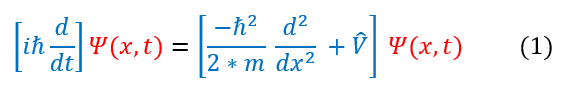
The Schrödinger Equation can be very difficult to solve (for the sole reason that wave functions for molecules can be huge even after approximations). Therefore, before we even get to solving quantum systems, let us first talk about common approximations made to the Schrödinger Equation to help solve these real problems. First let us remind ourselves what the Schrödinger Equation looks like:
By just looking at the equation above, one might notice that the time derivative and the positive derivative are on different sides of the equation. We previously discussed that having all time variables on one side and all position variables on the other side is a precursor for the standing wave approximation (which uses separation of variables). In order for this to be true we must have V(x,t) = V(x). This is actually true at equilibrium (the general state of an atomic system). Nevertheless, it is not always true. Hence we will be (generally) making these two postulates:
1. The potential is time independent (we have no changing potential field) and hence V(x,t) = V(x)
2. The particle is a standing wave and hence psi(x,t) = psi(x)*f(t)
These approximations can be modeled in the Schrödinger Equation below:
1. The potential is time independent (we have no changing potential field) and hence V(x,t) = V(x)
2. The particle is a standing wave and hence psi(x,t) = psi(x)*f(t)
These approximations can be modeled in the Schrödinger Equation below:
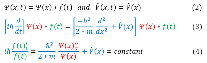
In order to make sure everyone is following, let us review some key steps below:
2: The explicit approximations we will make to the Schrödinger Equation
2 to 3: Adding the approximations from equation 2 into the Schrödinger Equation in equation 1
3 to 4: Dividing by psi(x) * f(t). Note: the f(t) in df(t)/dt cannot be canceled as we first need to take its derivative. Notice
that the LHS's value cannot change if I vary time (and not position). It equals a constant
We can note that in equation 4: psi(x) (the time independent wave function) must be a twice differentiable function and continuous.
Notation note: For clarity, I wrote df(t)/dt as f '_t. All I am saying in this notation is that it is a first derivative with respect to t. I am also doing the same notation for the x derivative.
Unit analysis will show that the constant must have units of energy. In fact, it does not look like we really changed the Schrödinger Equation at all besides the fact that the kinetic and potential energy only act on psi(x), while the total energy operator only acts on the f(t). We will therefore make another assumption:
3. The constant in equation 4 is the total energy
We can now solve the LHS of equation 4 below:
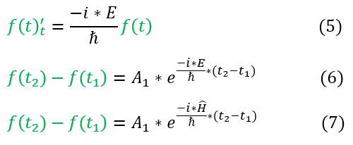
In order to make sure everyone is following, let us review some key steps below:
5: Rewriting the LHS of equation 4 with just the time terms and the constant
5 to 6: We solve the differential equation
6 to 7: E is the energy eigenvalue, which we can find through the Hamiltonian operator
For a free particle, the energy = h_bar * omega. While this is not the energy of every particle, the time dependent term is generally seen written with it added (noting that the omega now relates to the omega of the system evaluated and not necessarily E/h_bar). Equation 7 is commonly written, but, to be familiar with all versions, we replace E/h_bar below:
Note: we cannot fully solve the right hand side on the equation (the position dependent differential equation) as we need to know how V depends on x. The potential matters, and we will solve these systems in the next section of the course. For now, let us leave the position dependence as its most basic form (the sum of its basis functions phi(x)).
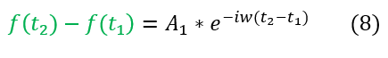
We are also allowed to start the time (t_1) whenever we want. It is easiest to set t_1 = 0, as then t_2 is just the total time t that has occurred. This leaves us with the final equation (for some w specific to the problem's angular frequency):
We are also allowed to start the time (t_1) whenever we want. It is easiest to set t_1 = 0, as then t_2 is just the total time t that has occurred. This leaves us with the final equation (for some w specific to the problem's angular frequency):
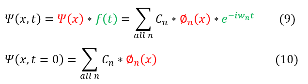
The above represents the formula for a psi(x,t). All we need to do is solve the phi(x). We can note that phi(x) is time independent and hence the same at t=0 and t=t. Hence, when we solve for phi(x), m we solve for the initial condition of psi(x,t=0). Time evolving each phi(x) in the basis will yield the time dependent wave function.
As we have just recently introduced a new operator (the Hamiltonian), let us note a few facts about the operator:
1. It is a real observable, hence the Hamiltonian is hermitian and equals its own adjoint.
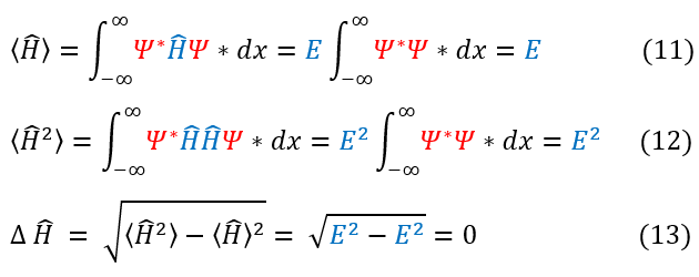
2. For a stationary state, the average energy is the eigenvalue of the Hamiltonian with 0 uncertainty.
We can check the second point by defining what a stationary state means. A stationary state is a constant energy state with no time dependent probability distribution. This means that the probability of all observables are time independent. The uncertainty in energy is shown below:
As we have just recently introduced a new operator (the Hamiltonian), let us note a few facts about the operator:
1. It is a real observable, hence the Hamiltonian is hermitian and equals its own adjoint.
2. For a stationary state, the average energy is the eigenvalue of the Hamiltonian with 0 uncertainty.
We can check the second point by defining what a stationary state means. A stationary state is a constant energy state with no time dependent probability distribution. This means that the probability of all observables are time independent. The uncertainty in energy is shown below:
|
|
|
