Now it is time to talk about one of the most fundamental classically forbidden experiments that led to the development of quantum mechanics. To be clear, the experiment was such a failure that it was coined the "UV catastrophe." This troubling physics is what is called black body radiation: radiation (light) produced from heating up an object (usually a metal). Think about a wire. A wire at room temperature appears grey or black; however, upon passing a current through (or placing the wire into a fire), it starts to glow bright red. From a physics perspective, if something glows a visible color, it must be emitting a certain wavelength of visible light. The only way known to emit light without burning an object was through the acceleration of electrons (see larmor radiation).
The classical picture at the time was as follows: electrons are bound to their respective atom in room temperature metals. When you heat up a metal, there is a continuous spectrum of electrons at all energies that start oscillating inside the metal. These oscillations (accelerations and de-accelerations) produce the electromagnetic radiation seen.
To model this picture, let us model electron oscillations like the particles on a string in "introduction to waves (The Wave Equation)." As each electron oscillates, it pulls the one adjacent to it up and down, creating a wave. We have previously modeled the wave using the wave equation below:
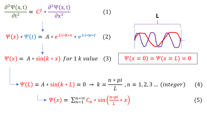
In order to make sure everyone is following, let us review some key steps below:
1 to 2: Previous, most general, solution to the wave equation.
2 to 3: At the end of the metal, we may assume that the electrons do not oscillate outs of the object. We therefore
impose a boundary condition on the wave disappears at x=0. e^(ikx) is a function composed of sin and cosine
terms. sin(0) = 0, but cos(0) = 1, so we can eliminate the cosine term from the e^(ikx) function.
3 to 4: The next boundary condition is that psi vanishes again at x = L. This is only true for certain k values.
4 to 5: Many different types of waves fit these two boundaries. For complete generalization, any combination of these
waves can be present at one time. The only non-constrained term is the C_n coefficient in front of every wave.
This 1-D wave oscillating in the x direction can also be generalized to 3-D by using separation of variables. If we approximate psi(x,y,z) as a standing wave, then it can be broken down to psi(x)*psi(y)*psi(z). Each psi(y) and psi(z) must satisfy the same boundary conditions as the 1 D wave for an LxLxL 3 D box. The standing wave inside the 3 D box is therefore as follows:
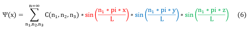
We can now plug this ansatz (guess) back into our wave equation to solve for the time portion psi(t).
In order to make sure everyone is following, let us review some key steps below:
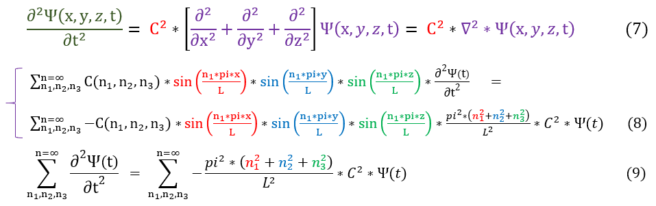
7: We can generalize the wave equation (see equation 1) to 3 dimensions by replacing the d^2/dx^2 with the laplacian.
7 to 8: We plugged in our ansatz into equation 7
8 to 9: similar terms are cancelled out.
This is a differential equation we can solve for any n_1, n_2, or n_3.
7: We can generalize the wave equation (see equation 1) to 3 dimensions by replacing the d^2/dx^2 with the laplacian.
7 to 8: We plugged in our ansatz into equation 7
8 to 9: similar terms are cancelled out.
This is a differential equation we can solve for any n_1, n_2, or n_3.
In order to make sure everyone is following, let us review some key steps below:
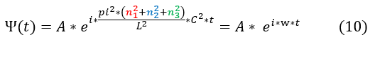
10: The solution to this differential equation is an e^i*theta(t) function. We also previous found it to be e^iwt.
We can now find the total amount of nodes (n_1^2+n_2^2+n_3^2) present in the LxLxL piece of metal. It is important to note that the boundary condition satisfied is for an oscillation across the whole LxLxL block; however, it could oscillate in between the block (without touching the edges). In order to account for these modes, we will take all the omega values possible from 0 to w.
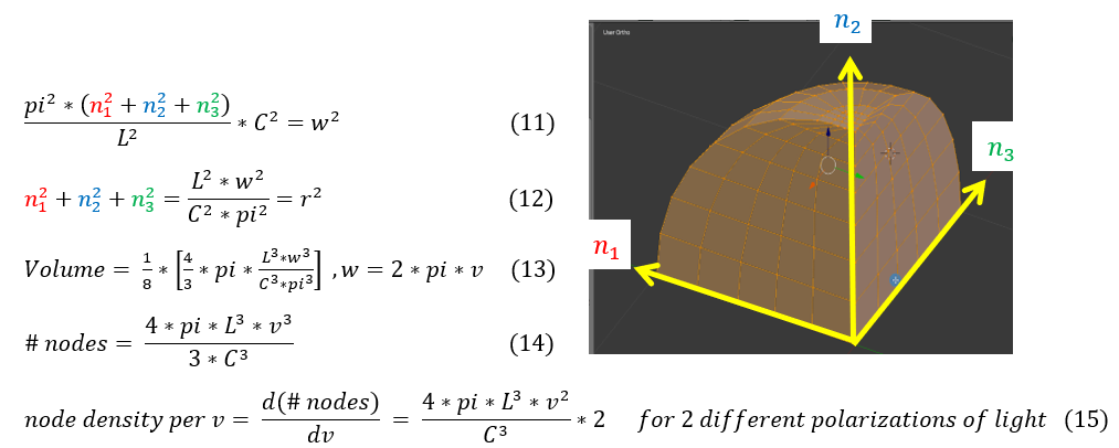
In order to make sure everyone is following, let us review some key steps below:
11: start from the maximum angular frequency for an oscillation from 0 to L across the metal
11 to 12: Solve for the total number of nodes. One can notice that for x=n_1 , y=n_2 , z=n_3 , this looks like a sphere
12 to 13: As the oscillations can at max go to frequency w, but at minimum be 0, we find the total amount of nodes by
taking the volume enclosed by the graph. n has to be positive, so we take the first octant volume.
13 to 14: replaced the angular frequency omega (w) to frequency of oscillation (v).
14 to 15: Electromagnetic radiation has 2 different polarization for an oscillating wave (rotate EM wave by 90
degrees). The node density (amount of nodes per frequency of oscillation) was calculated.
Now we have the amount of nodes for a given frequency of electron oscillation (and the hence the emitted light). The next question is, for a given frequency, what is the energy. HERE IS WHERE THE CLASSICAL PICTURE DIFFERS FROM THE QUANTUM MECHANICAL ONE.
Let us now look at the classical picture. In the classical picture, light can have a spectrum of energies. The probability of finding a photon at a certain energy is statistically interpreted through the Boltzmann distribution.
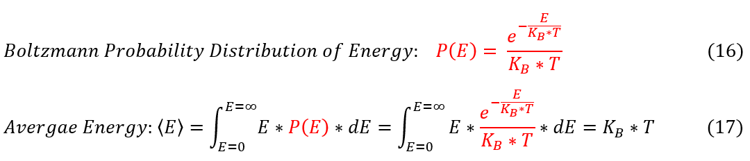
In order to make sure everyone is following, let us review some key steps below:
16: The Boltzmann distribution of energy
16 to 17: The weighted average energy = sum(all energy values * probability associated to each value)
With the average energy found, let us find the energy density (energy per volume) for the whole frequency spectrum.
16: The Boltzmann distribution of energy
16 to 17: The weighted average energy = sum(all energy values * probability associated to each value)
With the average energy found, let us find the energy density (energy per volume) for the whole frequency spectrum.
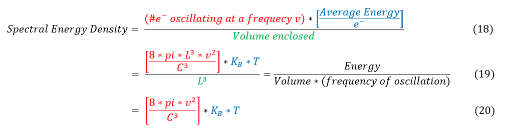
In order to make sure everyone is following, let us review some key steps below:
18: Linguistical definition of the spectral energy density
18 to 19: Plugging in the values previously found for each term.
19 to 20: Simplifying the expression.
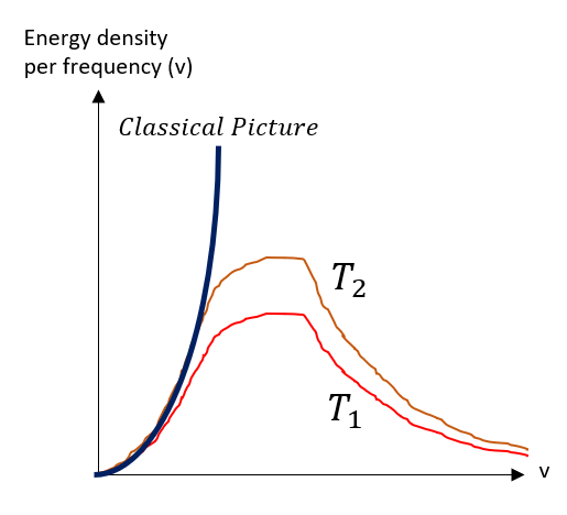
And with that, the physicists of the late 1800s were very sad. If you add up the whole spectra of energy, you will eventually diverge to infinity, but that is not what is observed. The graph below summarizes what was seen.
18: Linguistical definition of the spectral energy density
18 to 19: Plugging in the values previously found for each term.
19 to 20: Simplifying the expression.
And with that, the physicists of the late 1800s were very sad. If you add up the whole spectra of energy, you will eventually diverge to infinity, but that is not what is observed. The graph below summarizes what was seen.
|
For a T_2 > T_1, the picture does start going higher and higher, but it always converges down to zero. This does not make sense in the classical picture. Classically, the greater frequency of oscillation, the greater the energy should be and you just keep adding up all the energies possible.
Max Plank decided to do something drastic to fix this error. He made a very bold claim: light cannot exist at all energies. Through curve fitting, he found that this would make the graphs match if instead of a Boltzmann distribution (spectrum) of energies, photons can only exists at energies proportional to frequency (which was known to relate to energy). This proportionality factor is now called the plank''s constant = 6.626*10^(-34) J*sec |
Here are the new postulates made by Max Plank:
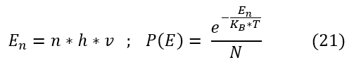
Where N = the normalization constant for the probability (all probabilities must sum to 1).
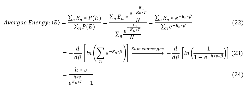
Now let us re-find the average energy with this new assumption:
Now let us re-find the average energy with this new assumption:
In order to make sure everyone is following, let us review some key steps below:
22: The new average energy, except instead of an infinitesimal sum (an integral), we take a discrete sum. beta = Kb*T
22 to 23: We rearrange the equation in the form of a derivative. This makes the sum easier to solve.
23 to 24: Taking the derivative yields us our final answer.
Let us now re-plug all the terms with our new average energy.
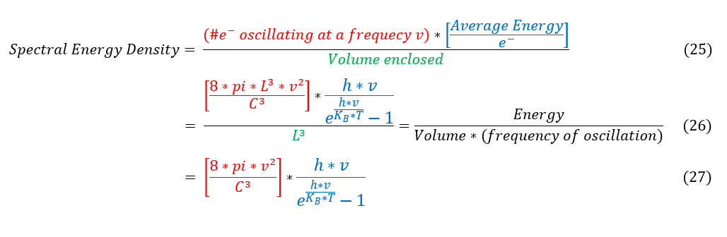
In order to make sure everyone is following, let us review some key steps below:
25: our old equation 18.
25 to 26: Plugging in the same values, but replacing the average energy term with our new solution.
26 to 27: Simplify to the new solution
For this new solution, it still follows the cubic growth for low frequency values, but now as frequency approaches infinity, the energy density converges to zero and follows the experimental data very well.
It should be noted that Max Plank believed that this was so coincidental he thought it was wrong. When Einstein used the constant to explain the photoelectric effect, he still was against the notion that his curve fitting was accurate.
The experiment of black body radiation teaches us that the energy of light is not a continuous spectrum, but appears at very discrete energies E = h*v.
|
|
|
