We have previously discussed the ability of a wave function to tunnel into a barrier, exponentially decaying on the way in. For wide barriers, this wave function will completely decay until zero, but one might have questioned: for thin enough barriers, can the wave function just pop out on the other side? The answer is, of course, YES! Let us pictorially represent what we are talking about:
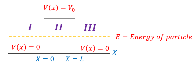
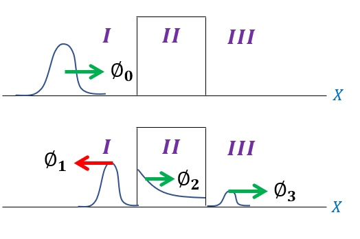
We will start with a wave function entering from the left hand side, with some of the basis states tunneling in + transmitting through and some reflecting back:
|
|
In order to make sure everyone is following, let us review some key steps below:
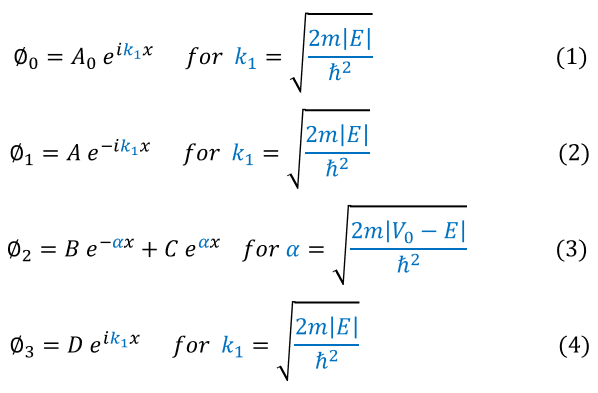
1: Phi_0 is moving in the positive x direction with an energy-potential gap of E
2: Phi_1 is moving in the negative x direction with an energy-potential gap of E
3: Phi_2 is moving in the positive x direction in a classically disallowed region
4: Phi_3 is moving in the positive x direction with an energy-potential gap of E
Note that wave functions do not actually move along the x axis until we time evolve them. Since we start the time evolution from -/+ infinity, we can notice that two wave functions starting at opposite sides on the x axis will exactly meet in the middle (at x = 0) if they have the same velocity. The velocity relates to the potential-energy gap; hence, phi_0 and phi_1 will have the same velocity and exactly meet at the same point in the middle when they are time evolved. Coincidentally, and follow carefully on this one, this is exactly the time were phi_0 vanishes (breaks up into phi_1 and phi_2) and phi_1 appears. Therefore, while it mathematically appears strange, we can physically describe the wave functions as so:
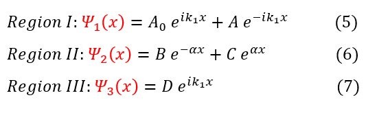
In order to make sure everyone is following, when time evolved, psi_1 may have two wave functions present, but they do NOT superimpose on each other as they start from opposite sides of the graph. Therefore, mathematically this really does describes the system (and we can just ignore A_1 and A_0 when we need to), but physically it does not. As the mathematical interpretation is what matters for now (with an understanding of how it relates to reality), we are fine to write this.
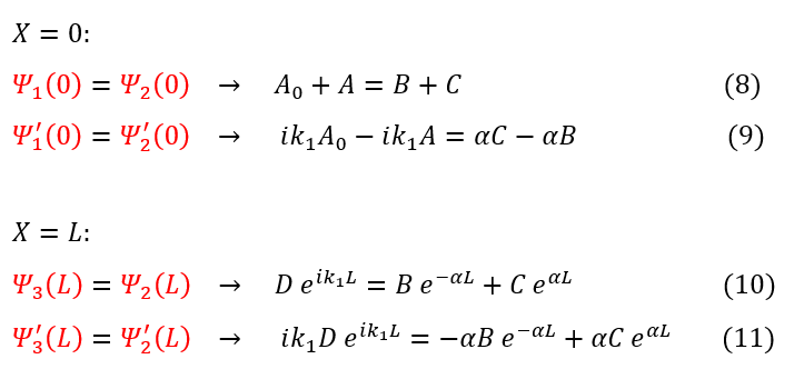
We can now go ahead and apply the boundary conditions at x = 0 and x = L:
1. No matter the potential, the wave function must be continuous
2. The slope of the wave function is only continuous for a finite potential barrier
We can now go ahead and apply the boundary conditions at x = 0 and x = L:
1. No matter the potential, the wave function must be continuous
2. The slope of the wave function is only continuous for a finite potential barrier
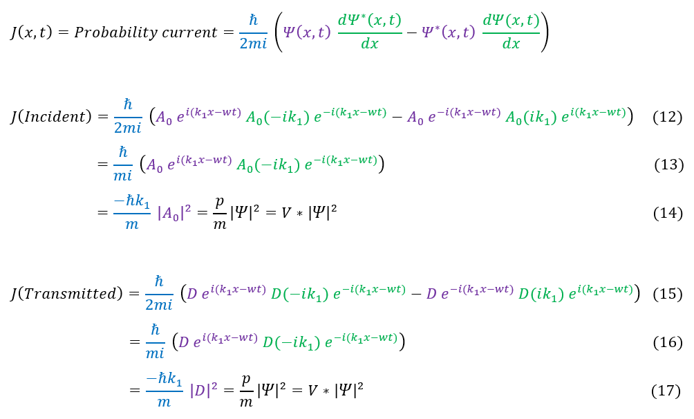
Remember, we can easily find the initial wave's A_0 value based on normalization. Therefore, we have 4 equations and 4 unknown, which is solvable, but we don't care about every variable (and it is a lot of math if one cares). What we care about is how much our probability distribution (wave function squared) makes it through the classically disallowed barrier (the probability a goldfish can swim out of its tank or a ball going through a wall). We are looking for the transmission coefficient:
In order to make sure everyone is following, let us review some key steps below:
12: Plug in the wave function for the incident wave into the continuity equation (Probability Current formula)
12 to 13: The two terms are the same and add together
13 to 14: The exponential term cancels out (magnitude 1).
The incident and transmission calculation are the same. Additionally, we also note that this reduces to our initial probability current definition for a plane wave: velocity * psi^2.
Therefore, the transmission coefficient of the wave through the barrier is:
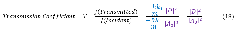
While we have 4 different equations with 4 unknowns, we really are only looking for D/A_0, We can now specifically solve for this ratio in a series of steps below. We need to get rid of A, B, and C:
In order to make sure everyone is following, let us review some key steps below:
8 and 9: Previous equations from the boundary conditions at x = 0
9 to 19: Subtitute in 'A' from equation 8
19 to 20: Get 'A_0' on one side (push 'B' and 'C' to the other side)
20 to 21: Group like terms
Now that we have gotten rid of 'A' we can now find a substitution for 'B' and 'C' in terms of 'D'
|
|
In order to make sure everyone is following, let us review some key steps below:
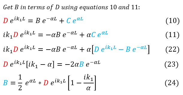
10 and 11: Previous equations from the boundary conditions at x = L
11 to 22: Replace 'C' with equation 10
22 to 23: Combine like terms (factor out 'D' and 'B')
23 to 24: Solve for 'B'
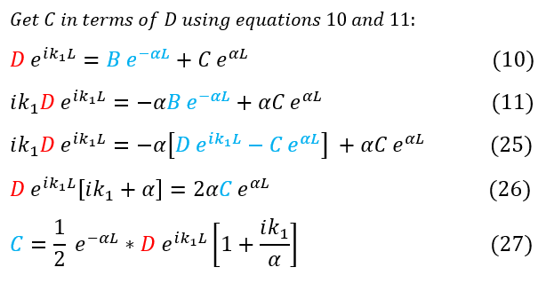
Equations 25-27 follow the same logic except we are solving for 'C'
Now that we have solved for 'B' and 'C' in terms of 'D' we can plug them back into equation 21 to get 'A_0' in terms of 'D.' Remember we want the ratio of D/A_0:
10 and 11: Previous equations from the boundary conditions at x = L
11 to 22: Replace 'C' with equation 10
22 to 23: Combine like terms (factor out 'D' and 'B')
23 to 24: Solve for 'B'
Equations 25-27 follow the same logic except we are solving for 'C'
Now that we have solved for 'B' and 'C' in terms of 'D' we can plug them back into equation 21 to get 'A_0' in terms of 'D.' Remember we want the ratio of D/A_0:
In order to make sure everyone is following, let us review some key steps below:
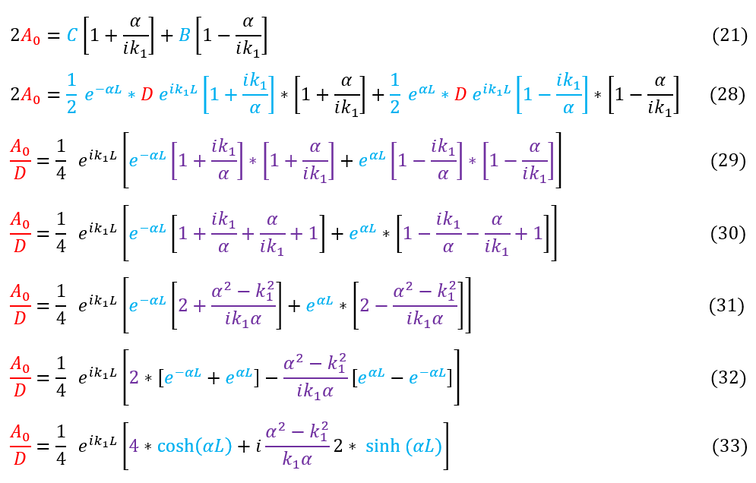
21 to 28: Plug in the expressions we found for 'B' and 'C'
28 to 29: Divide both sides by '2D' and factor out like terms
29 to 30: Expand the purple terms
30 to 31: Simplify the purple terms (combine the two fractions)
31 to 32: Reorder the terms. Factor out each purple terms in terms of the blue
32 to 33: One can now easily notice that the blue terms are hyperbolic sin and cosine
Now that we have the 'A_0/D' ratio, let us find the transmission coefficient:
In order to make sure everyone is following, let us review some key steps below:
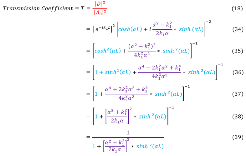
18 to 34: Plug in the ratio we found in equation 33
34 to 35: We take the magnitude squared. Note e^ik has a magnitude of 1 as we multiply by the complex conjugate
35 to 36: Expand the purple terms and replace cosh^2 with 1+sinh^2 (note the trig identities fro hyperbolic functions)
36 to 37: Combine sinh^2 terms
37 to 38: reduce the purple terms to a function squared
38 to 39: Write equation 38 as a fraction
And that is it. We have solved for the transmission coefficient for a wave function that tunnels through (E < V_0). Remember that 'alpha' and 'k' are actually functions of the energy and potential. Because it is actually more useful to have 'T' in terms of 'E' and 'V_0' let us rewrite the transmission coefficient below:
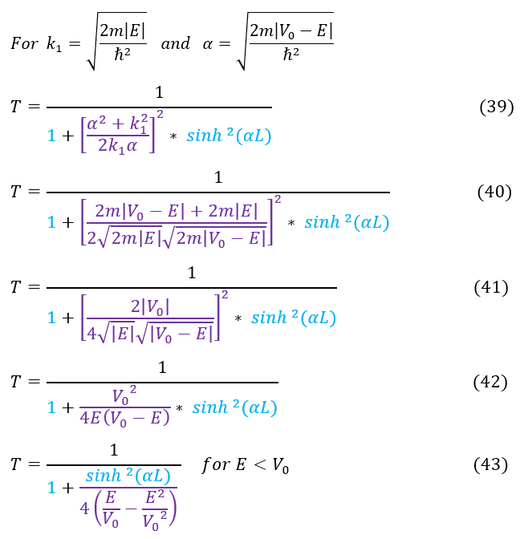
While it is a worthy exercise, it is worth noting that if E was greater than V_0 (scattering case instead of tunneling), we would have:
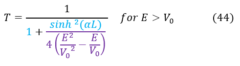
Additionally, for the curious folks, solving for the reflection coefficient would be extremely trivial as we could just use the relationship below:
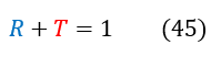
As good physicists, we should never just say we have our solution without checking our limiting cases (and dimensional analysis, but in this case it is obviously unitless). The limiting case we have is that for a huge potential-energy gap or a huge barrier (so big that the classically disallowed region's wave function decays to zero), our transmission frequency should be around or equal to zero. Restated: as 'alpha*L' -> infinity, T -> 0.
In order to make sure everyone is following, let us review some key steps below:
46: First we take the limit of sinh(alpha*L) as L goes to infinity
43 to 47: We use the limit in equation 46 and plug it into equation 43. Also, 1 is so much smaller than e^infinity
47 to 48: We rewrite the fraction in an easy to read format
48 to 49: This is a bunch of constants and e^-infinity which is just zero
And that is it! We have solved the tunneling problem for a constant potential (V_0 = constant). Equation 48 is commonly used as an approximation to the transmission formula, but it is important to note that this should be a very small number (in our limit).
|
|
|
