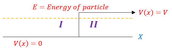
We can use these scatter state principles to reduce down to a 'half bound-state' example, where their is a finite barrier on one side of the well:
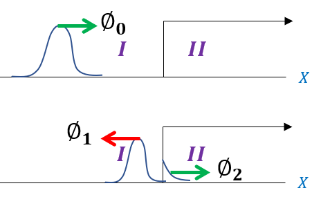
We will again start with a wave function entering from the left hand side, with some of the basis states tunneling in and some reflected back:
|
|
In order to make sure everyone is following, let us review some key steps below:
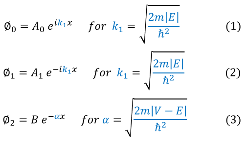
1: Phi_0 is moving in the positive x direction with an energy-potential gap of E
2: Phi_1 is moving in the negative x direction with an energy-potential gap of E
3: Phi_2 is moving in the positive x direction in a classically disallowed region
Note that wave functions do not actually move along the x axis until we time evolve them. Since we start the time evolution from -/+ infinity, we can notice that two wave functions starting at opposite sides on the x axis will exactly meet in the middle if they have the same velocity. The velocity relates to the potential-energy gap; hence, phi_0 and phi_1 will exactly meet at the same point in the middle when they are time evolved. Coincidentally, and follow carefully on this one, this is exactly the time were phi_0 vanishes (breaks up into phi_1 and phi_2) and phi_1 appears. Therefore, while it mathematically appears strange, we can physically describe the wave functions as so:
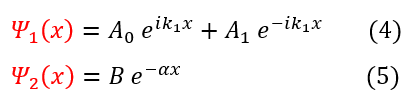
In order to make sure everyone is following, when time evolved, psi_1 may have two wave functions present, but they do NOT superimpose on each other as they start from opposite sides of the graph. Therefore, mathematically this describes the system (and we can just ignore A_1 and A_0 when we need to), but physically it does not. As the mathematical interpretation is what matters for now (with an understanding of how it relates to reality), we are fine to write this.
Before we go on and solve the problem, I just want to make one intuitive thing clear. Obviously, the wave function is tunneling a little, but it will eventually decay. In order to keep a normalized wave function in time, we should expect all the wave function to just bounce back (with equal and opposite velocity). With that intuition, let us go to the math.
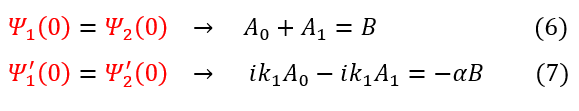
We can now go ahead and apply the boundary conditions:
1. No matter the potential, the wave function must be continuous
2. The slope of the wave function is only continuous for a finite potential barrier
Before we go on and solve the problem, I just want to make one intuitive thing clear. Obviously, the wave function is tunneling a little, but it will eventually decay. In order to keep a normalized wave function in time, we should expect all the wave function to just bounce back (with equal and opposite velocity). With that intuition, let us go to the math.
We can now go ahead and apply the boundary conditions:
1. No matter the potential, the wave function must be continuous
2. The slope of the wave function is only continuous for a finite potential barrier
Remember, we have solved for everything in the equation except for the A_1 and B normalization constants (we know the k values based on the energy-potential gap, and we know A_0 because of normalization).
We can now solve for A_1 and B in terms of A_0 by substituting them out of the equation:
We can now solve for A_1 and B in terms of A_0 by substituting them out of the equation:
|
|
In order to make sure everyone is following, let us review some key steps below:
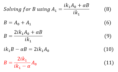
8: Solving for 'A_1' in equation 7
6 to 9: Plugging in equation 8 for 'A_1'
9 to 10: Multiplying both sides by 'iK_1' and subtracting 'alpha*B'
10 to 11: Solve for 'B'
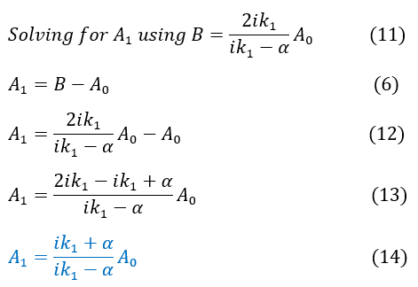
6 to 12: Plugging in equation 11 for 'B'
12 to 13: Factor out A_0 from the expression. Bring it all under one fraction
13 to 14: Simplify the numerator to get an expression for 'A_1'
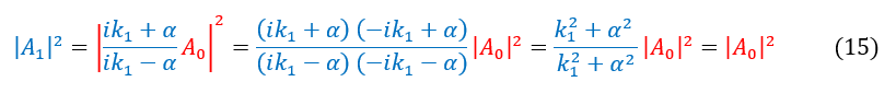
Now that we have solved for 'A_1' and 'B' we should now stop and check to see if this makes sense. In the end, the wave must be normalized at all times in this case. Since the tunneling decays eventually, we should expet A_0^2 and A_1^2 to be equal. We can check this below:
8: Solving for 'A_1' in equation 7
6 to 9: Plugging in equation 8 for 'A_1'
9 to 10: Multiplying both sides by 'iK_1' and subtracting 'alpha*B'
10 to 11: Solve for 'B'
6 to 12: Plugging in equation 11 for 'B'
12 to 13: Factor out A_0 from the expression. Bring it all under one fraction
13 to 14: Simplify the numerator to get an expression for 'A_1'
Now that we have solved for 'A_1' and 'B' we should now stop and check to see if this makes sense. In the end, the wave must be normalized at all times in this case. Since the tunneling decays eventually, we should expet A_0^2 and A_1^2 to be equal. We can check this below:
With that checked out, we can continue on. Now that we solved for every unknown variable, the next step is to calculate the transmission and reflection coefficients. In order to do this, we need to find the probability current (J-values) for the incident, reflected, and transmitted wave:
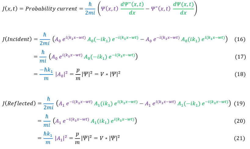
In order to make sure everyone is following, let us review some key steps below:
15: Plug in the wave function for the incident wave into the continuity equation (Probability Current formula)
15 to 16: The two terms are the same and add together
16 to 17: The exponential term cancels out (magnitude 1).
We also note that this reduces to our initial probability current definition for a plane wave: velocity * psi^2. Additionally The reflection calculation steps are identical to the incident one.
The Transmission coefficient calculation is slightly different (not a plane wave):
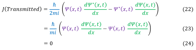
Any real wave has no probability current. We can now move forwards to calculate the reflection and transmission coefficients:
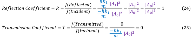
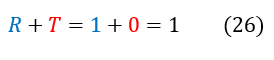
Just a conceptual check: the initial wave is split into two different waves; hence, T + R = 1 as the total fractional split must add up to one. We can check this below:
|
|
|
