In the last few pages of the course, we are going to focus on exactly solving the Hydrogen atom in quantum mechanics, one of the few fully solved problems in quantum. While it may at first seem shocking that we can exactly solve only a few problems with quantum mechanics, in the next course 'Quantum Mechanics II" we will discuss how we can use perturbation theory, variation theory, and Hartree-Fock to approximate any other solution. What we will see is that all of these perturbation approximations start from the Hydrogen atom's, as well as a few other, solution (so this is pretty important to understand).
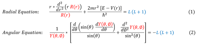
          To begin our discuss of solving the Hydrogen atom, let us remind ourselves of the two spherical Schrödinger equations we must solve (the radial and the angular):

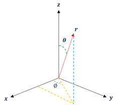
          It is important to note that even among scientists, people tend to define these coordinates differently. But as long as we are internally consistent, it is okay. To be clear, my coordinates are defined as follows:
       Theta: The angle the point makes with the z axis
       Phi: The angle the point makes with the x-axis in the x-y plane
       r: the distance between the point and the origin (Some call it 'Rho')

          For this page, we will focus our attention on solving the angular equation (we will solve the radial portion in the next one). To begin, we will make our separation of variables approximation for a standing wave:

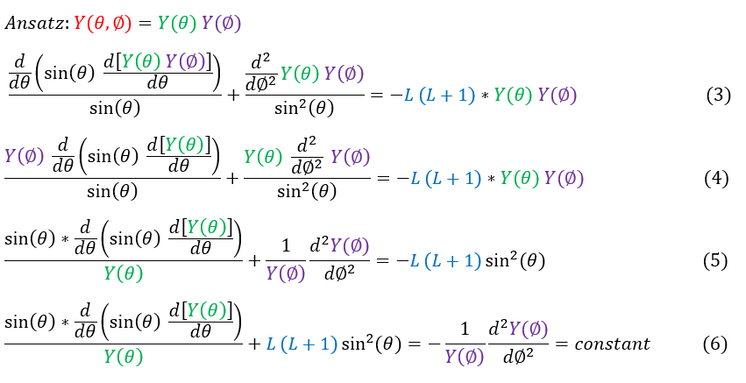
In order to make sure everyone is following, let us review some key steps below:
       3: We plug in our separation of variables ansatz (guess) into the angular equation (equation 2)
       3 to 4: We pull out Y(theta) and Y(phi) from the first and second term respectively as they are constant in the derivative
       4 to 5: We divide both sides by Y(phi) * Y(theta) and multiply by sin^2(theta)
       5 to 6: We push all the theta terms onto the LHS of the equation and the phi terms onto the RHS

          In equation 6, if the particle does not move in the theta directions at all, the LHS of the equation must be a constant. Since the LHS = the RHS of the equation, the RHS of the equation also must be a constant. Since this is a possibility, and the equation must hold for all possibilities, equation 6 must ALWAYS equal a constant. For now, we will conveniently call this constant m^2 (we will quickly see why we pick this constant). Let us focus our attention on solving the RHS of the equation:

In order to make sure everyone is following, let us review some key steps below:
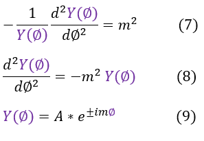
       7: The RHS of equation 6, setting the constant equal to m^2
       7 to 8: Multiply by - Y(phi)
       8 to 9: Solve the differential equation

          Hope fully equation 9 looks familiar because we have indeed already solved the Y(phi) wave function before in the Angular Momentum (Operators) page, equation 18. We can recall that the 'm' value actually does have significance. It is part of the eigenvalue of the 'Lz' operator.
          We can now focus our attention of the LHS, the theta portion, of the equation:

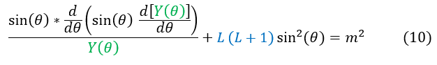
          One thing to notice about equation 10 is that the solution depends on the magnitude of 'm.' It does not differentiate between the positive and negative values.
          Now all we have to do is solve equation 10 to find the full angular solution to the Hydrogen atom. Unfortunately, it looks terribly ugly. One might start to cry trying to find a solution to this. Luckily, we keep around brilliant mathematicians just for this reason. Even before quantum mechanics, a mathematician named Adrien-Marie Legendre solved a similar problem, creating what are now known as Legendre polynomials. To solve this similar equation, we use what is now called the associated Legendre polynomial. Using the Legendre polynomials, the final form of the wave function is:

          We call the Y(theta, phi) the spherical harmonics (for it is the angular solution for a spherical potential). To solve the Legendre polynomials, we do need to input an 'L , m' value so we sometimes add a subscript to the 'Y.' Note that we did not need a potential to solve this equation here, but we did previously separate out the potential when we assumed that the potential was spherically symmetric (as it is for coulombic potential).

          Plugging in the full solution to the Legendre polynomials into the spherical harmonics (for a few different 'L , m' values) gets us:

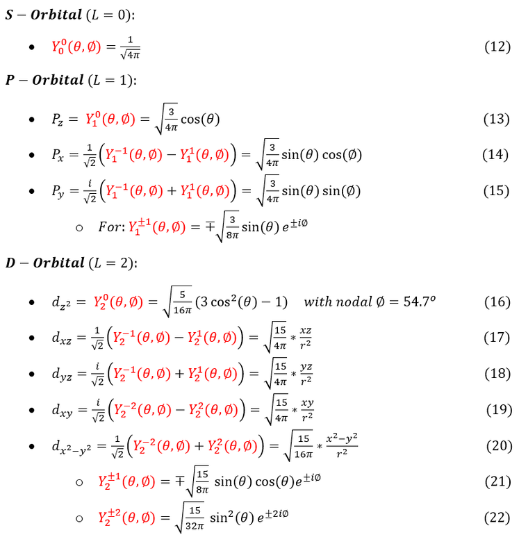
          Note that we have now labeled the different 'L' values to different orbital names. The orbital names are, in fact, quite arbitrary (made up). We are just now assigning these new names to these 'L' values we found. The 'L' value does tell us information about the angular momentum of the system, and hence these different orbitals have different angular momentum. The 'm' value tells us about the total angular momentum's z-orientation, leading to different orbital looks (which we subscript differently depending on the orbital's orientation).
          Some of the orbitals are linear combinations of spherical harmonic solutions. This is just a mathematical tool to find orthogonal harmonics (and we know that a linear combination of two solutions is always a solution). We needed to do this because our equation did not differentiate based on the +/- sign of 'm' (we could only find 1 solution, but needed two orthogonal ones, one for each value).
          I additionally reported some of the d-orbitals in Cartesian form. I only did this because I think it is more intuitive (in naming) when shown in this form. Converting back to spherical is pretty arbitrary.