|
|
|
Like for any quantum mechanics problem, once we define a potential we are now ready to solve the Schrödinger equation. This is not mathematically trivial (so prepare the tears). To ease future pain, we will define two new quantities to solve the Schrödinger equation (which may seem obvious for those who know the solution; However, for those who do not, remember that a brilliant mathematician / physicists solved this. I did not):
In order to make sure everyone is following, let us review some key steps below:
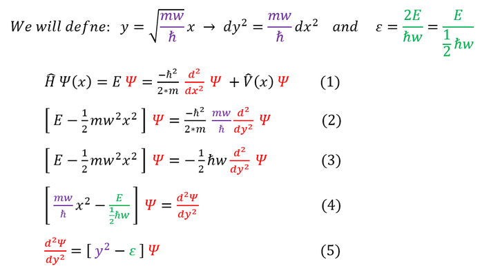
0: We define 2 new variables 'y' (unit length) and 'epsilon' (unit-less)
1: The general Schrödinger equation
1 to 2: Move V(x) onto the left side and plug in the harmonic oscillator potential. Replace d^2/dx^2 with d^2/dy^2
2 to 3: Simplify the right hand side
3 to 4: Divide both sides by -h_bar*w/2 (it is at this time, if one knows the answer, why we defined 'y' and 'epsilon')
4 to 5: Get the equation in terms of the variable 'y' and the constant 'epsilon'
This differential equation is less of a headache to solve (don't have to worry about tons of constants). In order to solve it, like any other differential equations, we need an ansatz (a trial function). In order to have a good anstaz, lets first get a general sense of the solution by looking at its extreme values (limiting cases): as y goes to infinity, the wave function psi(y) must go to zero. We can evaluate this limit below:
|
|
In order to make sure everyone is following, let us review some key steps below:
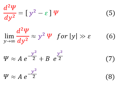
5: The Schrödinger equation in terms of the variable 'y' and the constant 'epsilon'
5 to 6: In the limit as 'y' goes to infinity, the constant 'epsilon' is essentially insignificant
6 to 7: An approximate solution to the new differential equation (in the limit a y goes to infinity)
7 to 8: The wave function must still normalize (decay at ends) as y goes to infinity, so we cannot have a exp(y^2) term
9: A check to see if we solved the differential equation in the limit as y goes to infinity
9 to 11: Take the first and second derivative
11 to 12: As 'y' goes to infinity, 'A*y^2' is so much bigger than 'A', such that 'A' is insignificant
12 to 13: We can now see that this is the solution to the differential equation in the limit as y goes to infinity
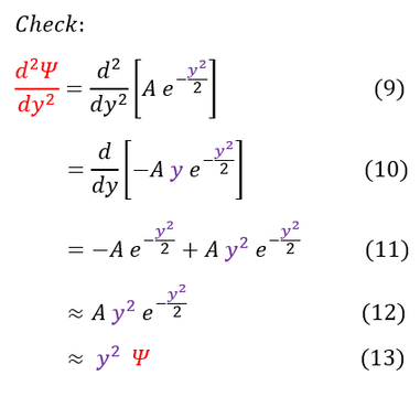
We now have a general idea of how the solution acts as 'y' goes to +/- infinity. As 'y' goes to +/- infinity, the exponential term dominates the value of psi. However, as 'y' becomes smaller and smaller, the co-factor 'A' is no longer an insignificant value. While it may have acted like a constant in the limit, it could possibly vary with 'y.' We can account for that in our new general ansatz below:
5: The Schrödinger equation in terms of the variable 'y' and the constant 'epsilon'
5 to 6: In the limit as 'y' goes to infinity, the constant 'epsilon' is essentially insignificant
6 to 7: An approximate solution to the new differential equation (in the limit a y goes to infinity)
7 to 8: The wave function must still normalize (decay at ends) as y goes to infinity, so we cannot have a exp(y^2) term
9: A check to see if we solved the differential equation in the limit as y goes to infinity
9 to 11: Take the first and second derivative
11 to 12: As 'y' goes to infinity, 'A*y^2' is so much bigger than 'A', such that 'A' is insignificant
12 to 13: We can now see that this is the solution to the differential equation in the limit as y goes to infinity
We now have a general idea of how the solution acts as 'y' goes to +/- infinity. As 'y' goes to +/- infinity, the exponential term dominates the value of psi. However, as 'y' becomes smaller and smaller, the co-factor 'A' is no longer an insignificant value. While it may have acted like a constant in the limit, it could possibly vary with 'y.' We can account for that in our new general ansatz below:
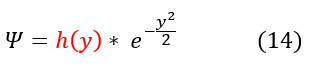
Where h(y) is some function of 'y'. We can now plug back in our ansatz to solve for h(y):
In order to make sure everyone is following, let us review some key steps below:
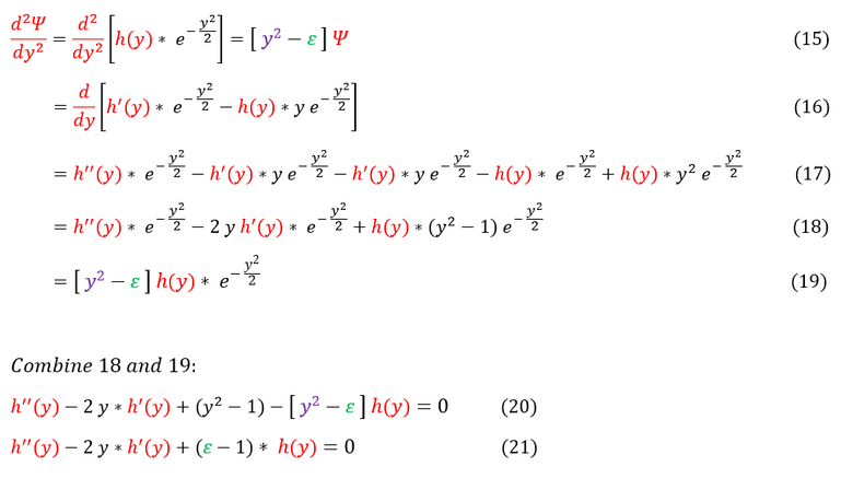
15: Plug our ansatz into equation 5 (the Schrödinger equation)
15 to 17: Only the LHS shown. Take the first and second derivative of the ansatz (psi)
17 to 18: Simplify the expression
18 to 19: Reshow the RHS of the equation with the ansatz plugged in
19 to 20: Combine the LHS (equation 18) and the RHS (equation 19). We also cancel out the exp(-y^2) term
20 to 21: Simplify the expression
We now have a second order differential equation for the h(y) function. In order to solve a differential equation (just like before) we need another ansatz. This time, we will expand out h(y) into a polynomial series (see power series for reference). For those unfamiliar with this trick, it is the same principle of Taylor series. We will show this below:
In order to make sure everyone is following, let us review some key steps below:
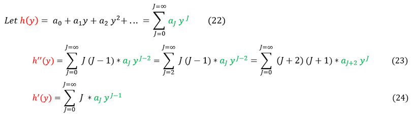
22: The definition of a power series
23 and 24: We apply the derivatives on the power series. For equation 23, we reformat the indeces (see below)
Note the switch in indeces for equation 23. We do this because when J = 0 and 1 we are adding zero in our sum (which is trivial). We therefore switch the index to the first non-zero term being summed, which is J = 2. However, because we want to combine all of these summations, we need to sum over the same index. When we switch back to start from J = 0, we really mean the 2nd index. To mathematically equate the two indeces, we add 2 to all J terms.
Let us now plug this ansatz into equation 21 to solve for the 'a_J' terms in the polynomial expansion of h(y):
In order to make sure everyone is following, let us review some key steps below:
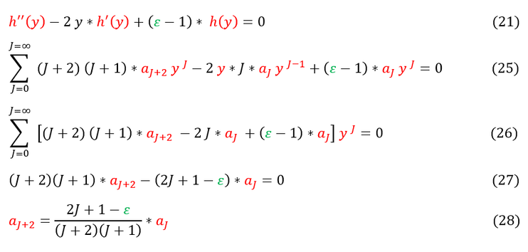
21: Our differential equation we need to solve for h(y)
25: Plug in our power series expansion of h(y) (see equations 22 - 24)
25 to 26: Factor out a y^J
26 to 27: 'y' (a function of 'x') spans from +/- infinity. Hence, its coefficient must sum to zero at all 'y' values / indeces
27 to 28: Solve for 'a_j+2' in terms of 'a_j'
The first thing to notice about equation 28 is that we need two inputs to solve for every 'a_j' value (we need an even input and an odd input). This should make sense as we have a second order differential equation, which requires two initial conditions to solve.
Some mathematicians might immediately see the problem with equation 28. However, it is not immediately obvious, so lets make it clear. Let us look at the limiting case as J goes to infinity (the last terms in the infinite summation):
|
|
In order to make sure everyone is following, let us review some key steps below:
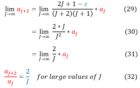
29: Finding 'a_J+2' for large values of 'J' (as J goes to infinity)
29 to 30: Constants in the numerator and order(1) terms in the denominator are insignificant in the limit
30 to 31: Simplify the expression
31 to 32: We find The ratio of 'a_j+2' to ''a_j' to be 2/J
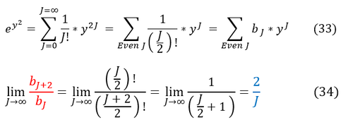
33: We can Taylor expand exp(y^2) into a format that matches the power series starting equation (for 'b' instead of 'a')
33 to 34: Now when we take the ratio, in the limit as J goes to infinity, we again find the same ratio 2/J
For very large 'J' values, our expression in equation 28 acts like exp(y^2). This is NOT good because, going back to the beginning, we MUST have the wave function normalize. If h(y) has an exp(y^2) term then:
29: Finding 'a_J+2' for large values of 'J' (as J goes to infinity)
29 to 30: Constants in the numerator and order(1) terms in the denominator are insignificant in the limit
30 to 31: Simplify the expression
31 to 32: We find The ratio of 'a_j+2' to ''a_j' to be 2/J
33: We can Taylor expand exp(y^2) into a format that matches the power series starting equation (for 'b' instead of 'a')
33 to 34: Now when we take the ratio, in the limit as J goes to infinity, we again find the same ratio 2/J
For very large 'J' values, our expression in equation 28 acts like exp(y^2). This is NOT good because, going back to the beginning, we MUST have the wave function normalize. If h(y) has an exp(y^2) term then:
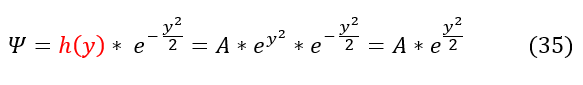
exp(1/2*y^2) does NOT normalize and cannot be how our equation acts as y goes to +/- infinity.
The only way to mathematically get around this fact is if we NEVER sum up these diverging terms. We need our summation to converge (as our wave function should never diverge to infinity); hence, we need 'a_j+2' to go to zero at one point. Once 'a_j+2' = 0 , the rest of the terms in the infinite summation also equals zero and the finite summation will converge.
The only way to mathematically get around this fact is if we NEVER sum up these diverging terms. We need our summation to converge (as our wave function should never diverge to infinity); hence, we need 'a_j+2' to go to zero at one point. Once 'a_j+2' = 0 , the rest of the terms in the infinite summation also equals zero and the finite summation will converge.
In order to make sure everyone is following, let us review some key steps below:
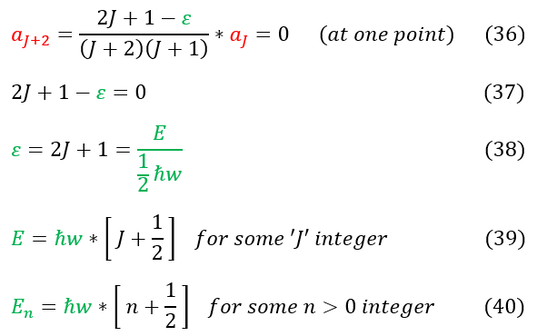
36: Equation 28 (relationship between 'a' coefficients in the power series). For some J_max, 'a_j+2' must be zero
36 to 37: Simplify the expression
37 to 38: Solve for 'epsilon' and plug in our initial expression for 'epsilon' (top of page)
38 to 39: Solve for the energy 'E'
39 to 40: Equation commonly seen with 'n' (same as 'J': an index). Energy cannot be zero; 'n' must be greater than zero
And that is the energy of the quantum harmonic oscillator. Note that 'n' values only go up to some 'n_max' (except the harmonic oscillator is only valid for small perturbations anyways). There are two very important notes about energy:
1. The ground state energy 'n' = 0 (even) is not zero energy (as nothing has zero energy), but rather 1/2*h_bar*w
2. All energy levels are evenly spaced by some constant h_bar*w (energy is quantized)
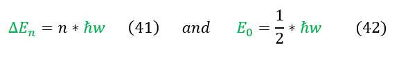
This energy quantization mathematically arose because of the necessity for the series to converge (for the wave function to be normalized). Because not all wave functions normalize, not all energies are possible (remember, this is similar to the particle in a box situation / energy quantization). We can represent these two facts below:
36: Equation 28 (relationship between 'a' coefficients in the power series). For some J_max, 'a_j+2' must be zero
36 to 37: Simplify the expression
37 to 38: Solve for 'epsilon' and plug in our initial expression for 'epsilon' (top of page)
38 to 39: Solve for the energy 'E'
39 to 40: Equation commonly seen with 'n' (same as 'J': an index). Energy cannot be zero; 'n' must be greater than zero
And that is the energy of the quantum harmonic oscillator. Note that 'n' values only go up to some 'n_max' (except the harmonic oscillator is only valid for small perturbations anyways). There are two very important notes about energy:
1. The ground state energy 'n' = 0 (even) is not zero energy (as nothing has zero energy), but rather 1/2*h_bar*w
2. All energy levels are evenly spaced by some constant h_bar*w (energy is quantized)
This energy quantization mathematically arose because of the necessity for the series to converge (for the wave function to be normalized). Because not all wave functions normalize, not all energies are possible (remember, this is similar to the particle in a box situation / energy quantization). We can represent these two facts below:
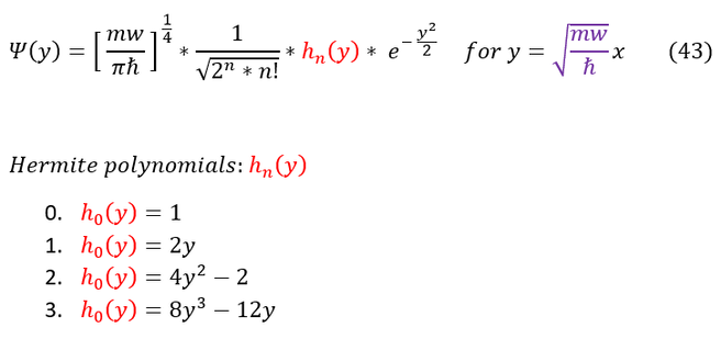
The last thing to do is to finish solving the wave function of the quantum harmonic oscillator (sometimes abbreviated as QHO). One might start to cry trying to find a solution to this. Luckily, we keep around brilliant mathematicians just for this reason. Even before quantum mechanics, mathematicians like Laplace and Chebyshev (very famous people) already worked out what is now called Hermite polynomials. The solution to the quantum harmonic oscillator trends just like a Hermite polynomial (as a physicists you shouldn't be expected to see this, but you can look more into the polynomials ... they have many applications even outside of physics). Using the Hermite polynomials, the final form of the wave function is:
And that is the brute force way of solving the quantum harmonic oscillator for some 'n' index (first excited state, second excited state; we know that 'n' index's energy states as 'n' is directly proportional to energy). The next page will discuss the much easier and simpler way using ladder operators (but it is good to see the math version first). Before we continue, let us discuss a couple pitfalls when it comes to the quantum harmonic oscillator.
1. In reality, energy levels are NOT evenly spaced by h_bar*w. The quantum harmonic oscillator approximates (very well) local energy minimums, but we are assuming some sort of beautiful symmetry. In real perturbed systems, the energy spacing gets smaller and smaller as one goes up.
2. At some point, the electron or atom may have enough energy to be unbound from the potential well / restorative force (it will get over the energy barrier). This is not predicted in the harmonic oscillator because the harmonic oscillator assumes a bounded well at any energy level.
3. Do NOT confuse physciist's Hermite polynomials with other versions of them (make sure the trend matches the ones above as their are many versions of Hermite polynomials as their are different applications)
In conclusion, remember that the harmonic oscillator is only a good approximation for small oscillations although people tend to apply it to many systems to explain quantum behavior. It provides us with a good intuition of how the particle behaves at a local minimum, but remember its limitations.
|
|
|
