Heisenberg's Uncertainty Principle was a defining moment in quantum mechanics. It mathematically defines that, no matter how well an experiment is run, some observables can never be known with certainty at the same time. In contrast, in Newtonian mechanics, the uncertainty in a measurement rests entirely in the experimental setup. To prove and understand this principle, let us first take a look at the Shwartz inequality:
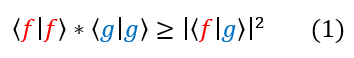
When I first introduced Dirac notation, I made a slight note about its resemblance to an inner product. In fact, it is based off the same principles (besides the operator part). Inner product tells us how parallel 2 vectors / functions are (0 for orthogonal functions with a maximum value for parallel functions). The maximum overlap two functions can have is in fact with itself. Hence, the inner products of <f,f> and <g,g> will always be bigger than or the same as the square of f and g's overlap with each other.
We can use this principle with the product of the variance of two operators:
We can use this principle with the product of the variance of two operators:
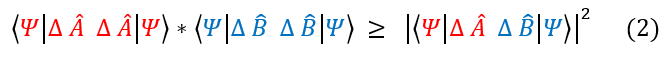
Here we are just replacing f with A | psi > and g with B | psi >. We can now break down the inner part of the Dirac notation on the right hand side ( < psi | ΔA ΔB | psi > ) into its most general form: real and imaginary parts.
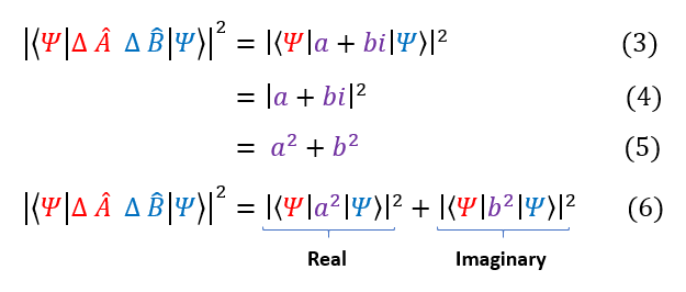
Let us now evaluate both the real and imaginary parts of ΔA ΔB
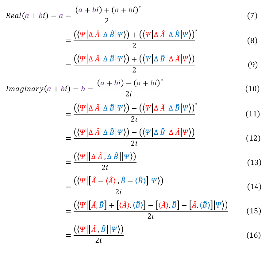
In order to make sure everyone is following, let us review some key steps below:
7: The definition of how to isolate the real part of a function
7 to 8: Our function plugged into the equation
8 to 9: Took the complex conjugate. Remember, the bra on the left is complex conjugated and the ket is not. When we
add our own complex conjugate to the system, to keep Dirac notation, we must switch the bra and the ket.
10: The definition of how to isolate the imaginary part of a function
10 to 11: Our function plugged into the equation
11 to 12: Took the complex conjugate. Remember, the bra on the left is complex conjugated and the ket is not. When
we add a complex conjugate to the system, to keep Dirac notation, we must switch the bra and the ket.
12 to 13: We notice that this is the definition of a commutator relation.
13 to 14: We plug in the deifnition of the uncertainty
14 to 15: Expand the commutator
15 to 16: The average value ( <A> ) of any operator is a scalar and scalars commute (commutator=0) with everything
To recap, the real part gave us an anti-commutator (AB + BA), while the imaginary part gave us a commutator (AB - BA). We may also note that the uncertainties in A and B are always positive; hence, the real part is always positive. Since we are already calculating the minimum of a function, we can throw away the real part (this will just make our bound even more strict).
In order to make sure everyone is following, let us review some key steps below:
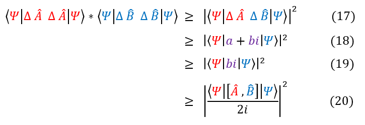
17: Our original equation we were evaluating in equation 2.
18: The most general form of any scalar is a + bi
18 to 19: We proved that a will always be positive. Hence, the inequality holds without a (9 > 1 + 3 and 9 > 3 )
19 to 20: Plugged in the expression we found for the imaginary part from equation 16.
And this concludes the proof of the Heisenberg's Uncertainty Principle. The full form is simplified below:
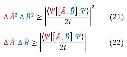
Note that the product of the two uncertainties is always real and positive.
It is now time to interpret this result. The only way the product of the two uncertainties equals zero is if the two operators commute. The only way the commutator equals zero is if the two operators share at least one eigenfunction with each other (for on that eigenfunction, the operators would just scale the function and not change it). Hence, The only way for the product of two uncertainties to be zero is if the operator shares at least one eigenfunction.
Note that if an eigenfunction is shared, then it does not necessarily mean that the operators commute! It is not a two way relation. One example is the position and momentum operators. Both share the basis e^ikx, but they do not commute.
Let us now see the importance of this statement. If two operators do not commute, than an uncertainty relationship hold. Then, regardless of the experimental apparatus, we can NEVER know both quantities with certainty at the same time. Some observes can never be known at the exact same time.
Let us walk through a very common example to solidify this:
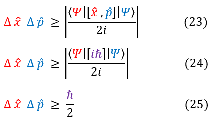
In order to make sure everyone is following, let us review below:
23: The Heisenberg's Uncertainty Principle for x and p
23 to 24: Plugged in the commutator for x and p
24 to 25: Simplified the expression
Hence, I can NEVER now a particle's position and momentum in quantum mechanics at the same time. If I did happen to know, with certainty, a particle's position, then we would have:
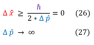
If we did know position with 100 % certainty, then we would have to be 0 % sure about momentum to not violate the Heisenberg's Uncertainty Principle. In fact, this is what we observe. The wave function with 100 % certainty in position is a delta function centered at some position (if we know the position with 100 % certainty, then the probability wave has to reduce to zero everywhere except at that one location). However, if we are in a delta function, then we have no knowledge whatsoever what the k value of the wave is ( which is bad since p = h_bar * k ). Hence, we have zero clue what the momentum is at that exact moment. Once we remeasure the momentum, we now loose all information about the position.
We can only have certainty for two observables in our experiments if their two corresponding operators commute.
|
|
|
