|
|
|
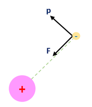
A one electron atom consists only of a nucleus and a sole electron. The electron is held (bounded) by the nucleus by an electrostatic interaction (a radial force). Our quantum picture of this system is diagrammed below:
|
|
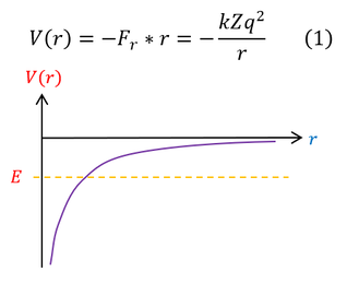
Where k = Coulomb constant; Z = nuclear charge; q = charge of a lone electron or proton
In the diagram, we only show the electron moving. This is because the nuclear mass is much bigger than the electron's mass, and hence, for the same force, the electron accelerates and moves a lot more. It moves so much, that the nuclear movements are rather negligible in comparison (we don't really see the nucleus move that much). We call this the Born-Oppenheimer approximation (and sometimes the Franck-Condon limit depending on your field). Regardless, the Schrödinger equation does not differentiate on this basis, but I thought I would point this out.
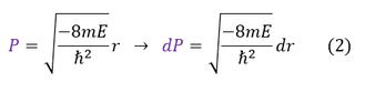
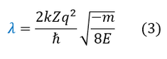
What is important to solve is the Schrödinger equation and for that we need the potential energy. From non-relativistic electromagnetism, we know the force and potential energy exerted on two charged particles (shown in the above diagram on the right). Electrostatic forces are considered radial forces, which is a spherically symmetric force / potential. Therefore, all we need to do is solve the radial and angular equations we found earlier. In this page we will focus on the radial wave equation for the S-orbital (L = 0) for any 1-electron atom of charge 'Z.' It will be a mathematically challenging equation, so we will make 3 simplifying substitutions to our radial wave equation:
In the diagram, we only show the electron moving. This is because the nuclear mass is much bigger than the electron's mass, and hence, for the same force, the electron accelerates and moves a lot more. It moves so much, that the nuclear movements are rather negligible in comparison (we don't really see the nucleus move that much). We call this the Born-Oppenheimer approximation (and sometimes the Franck-Condon limit depending on your field). Regardless, the Schrödinger equation does not differentiate on this basis, but I thought I would point this out.
What is important to solve is the Schrödinger equation and for that we need the potential energy. From non-relativistic electromagnetism, we know the force and potential energy exerted on two charged particles (shown in the above diagram on the right). Electrostatic forces are considered radial forces, which is a spherically symmetric force / potential. Therefore, all we need to do is solve the radial and angular equations we found earlier. In this page we will focus on the radial wave equation for the S-orbital (L = 0) for any 1-electron atom of charge 'Z.' It will be a mathematically challenging equation, so we will make 3 simplifying substitutions to our radial wave equation:
|
|

|
We can now plug these into the radial equation:
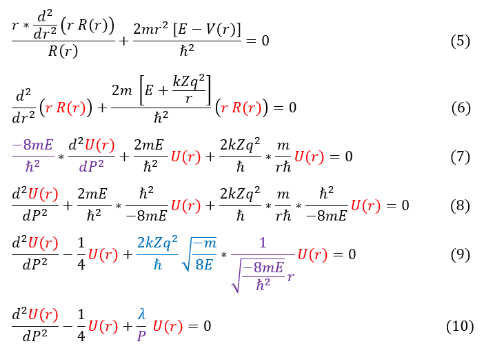
In order to make sure everyone is following, let us review some key steps below:
5: The radial Schrödinger equation for L = 0
5 to 6: Multiply by R(r) / r and plug in our radial potential
6 to 7: Distribute out the parenthesis and replace dr^2 with dP^2
7 to 8: Divide out the purple term
8 to 9: Simplify the middle term and reorganize the right term to match equations 2 and 3
9 to 10: Plug in equations 2 and 3
This differential equation is less of a headache to solve (don't have to worry about tons of constants). In order to solve it, like any other differential equations, we need an ansatz (a trial function). In order to have a good anstaz, lets first get a general sense of the solution by looking at its extreme values (limiting cases): as r (and by extension P) goes to infinity, the wave function R(r) (and by extension U(r)) must go to zero. We can evaluate this limit below:
|
|
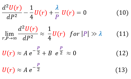
In order to make sure everyone is following, let us review some key steps below:
10: Our equation we are trying to solve
10 to 11: We take the limit of the equation as r (or P) goes to infinity (1/P is now essentially zero)
11 to 12: We solve the differential equation
12 to 13: As P goes to infinity, U(r) must go towards zero, which cannot happen with the 'B' term; hence, B must be zero
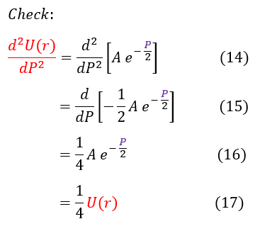
We do a quick mathematical check on the right to make sure we solved the differential equation correctly.
We now have a general idea of how the solution acts as 'r' or 'P' goes to +/- infinity. As 'P' goes to +/- infinity, the exponential term in equation 13 dominates the value of U(r). However, as 'P' becomes smaller and smaller, the co-factor 'A' is no longer an insignificant value. While it may have acted like a constant in the limit, it could possibly vary with 'P.' We can account for that in our new general ansatz below:
10: Our equation we are trying to solve
10 to 11: We take the limit of the equation as r (or P) goes to infinity (1/P is now essentially zero)
11 to 12: We solve the differential equation
12 to 13: As P goes to infinity, U(r) must go towards zero, which cannot happen with the 'B' term; hence, B must be zero
We do a quick mathematical check on the right to make sure we solved the differential equation correctly.
We now have a general idea of how the solution acts as 'r' or 'P' goes to +/- infinity. As 'P' goes to +/- infinity, the exponential term in equation 13 dominates the value of U(r). However, as 'P' becomes smaller and smaller, the co-factor 'A' is no longer an insignificant value. While it may have acted like a constant in the limit, it could possibly vary with 'P.' We can account for that in our new general ansatz below:
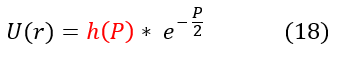
Where h(P) is some function of 'P' we don't know yet. We can now plug back in our ansatz to equation 10 to solve for h(P):
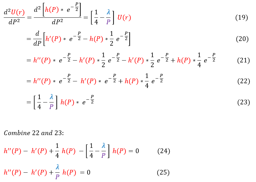
In order to make sure everyone is following, let us review some key steps below:
19: Plug our ansatz into equation 10
19 to 21: Only the LHS shown. Take the first and second derivative of the ansatz (psi)
21 to 22: Simplify the expression
22 to 23: Reshow the RHS of the equation with the ansatz plugged in
24: Combine the LHS (equation 22) and the RHS (equation 23). We also cancel out the exp(-P/2) terms
24 to 25: Simplify the expression
We now have a second order differential equation for the h(P) function. In order to solve a differential equation (just like before) we need another ansatz. This time, we will expand out h(P) into a polynomial series (see power series for reference). For those unfamiliar with this trick, it is the same principle of Taylor series. We will show this below:
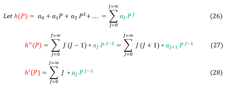
In order to make sure everyone is following, let us review some key steps below:
26: The definition of a power series
27 and 28: We apply the derivatives on the power series. For equation 27, we reformat the indeces (see below)
Note the switch in indeces for equation 27. We do this because when J = 0 we are adding zero in our sum (which is trivial). We therefore skip over this index in the summation as it is just adding in zero. In order to do this, we add 1 to ever J term.
Let us now plug this ansatz into equation 25 to solve for the 'a_J' terms in the polynomial expansion of h(P):
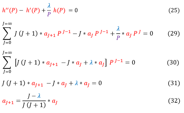
In order to make sure everyone is following, let us review some key steps below:
25: Our differential equation we need to solve for h(P)
29: Plug in our power series expansion of h(P) (see equations 26 - 28)
29 to 30: Factor out a P^J
30 to 31: 'P' (a function of 'r') spans from +/- infinity. Hence, its coefficient must sum to zero at all 'P' values / indeces
31 to 32: Solve for 'a_j+1' in terms of 'a_j'
Some mathematicians might immediately see the problem with equation 32. However, it is not immediately obvious, so lets make it clear. Let us look at the limiting case as J goes to infinity (the last terms in the infinite summation):
25: Our differential equation we need to solve for h(P)
29: Plug in our power series expansion of h(P) (see equations 26 - 28)
29 to 30: Factor out a P^J
30 to 31: 'P' (a function of 'r') spans from +/- infinity. Hence, its coefficient must sum to zero at all 'P' values / indeces
31 to 32: Solve for 'a_j+1' in terms of 'a_j'
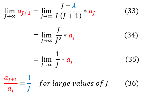
Some mathematicians might immediately see the problem with equation 32. However, it is not immediately obvious, so lets make it clear. Let us look at the limiting case as J goes to infinity (the last terms in the infinite summation):
|
|
In order to make sure everyone is following, let us review some key steps below:
33: Finding 'a_J+1' for large values of 'J' (as J goes to infinity)
33 to 34: Constants in the numerator and order(1) terms in the denominator are insignificant in the limit
34 to 35: Simplify the expression
35 to 36: We find The ratio of 'a_j+1' to ''a_j' to be 1/J
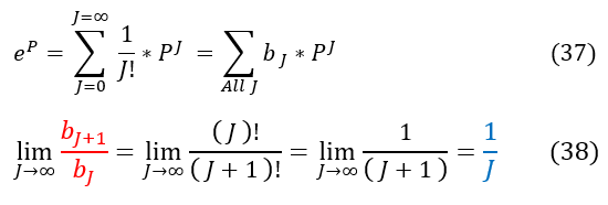
37: We can Taylor expand exp(P) into a format that matches the power series starting equation (for 'b' instead of 'a')
37 to 38: Now when we take the ratio, in the limit as J goes to infinity, we again find the same ratio 1/J
For very large 'J' values, our expression in equation 36 acts like exp(P). This is NOT good because, going back to the beginning, we MUST have the wave function normalize. If h(P) has an exp(P) term then:
33: Finding 'a_J+1' for large values of 'J' (as J goes to infinity)
33 to 34: Constants in the numerator and order(1) terms in the denominator are insignificant in the limit
34 to 35: Simplify the expression
35 to 36: We find The ratio of 'a_j+1' to ''a_j' to be 1/J
37: We can Taylor expand exp(P) into a format that matches the power series starting equation (for 'b' instead of 'a')
37 to 38: Now when we take the ratio, in the limit as J goes to infinity, we again find the same ratio 1/J
For very large 'J' values, our expression in equation 36 acts like exp(P). This is NOT good because, going back to the beginning, we MUST have the wave function normalize. If h(P) has an exp(P) term then:
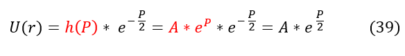
exp(P/2) does NOT normalize and cannot be how our equation acts as P (or r) goes to +/- infinity.
The only way to mathematically get around this fact is if we NEVER sum up these diverging terms at all. We need our summation to converge (as our wave function should never diverge to infinity); hence, we need 'a_j+1' to go to zero at one point. Once 'a_j+1' = 0 , the rest of the terms in the infinite summation also equals zero and the finite summation will converge (not go to infinity)
The only way to mathematically get around this fact is if we NEVER sum up these diverging terms at all. We need our summation to converge (as our wave function should never diverge to infinity); hence, we need 'a_j+1' to go to zero at one point. Once 'a_j+1' = 0 , the rest of the terms in the infinite summation also equals zero and the finite summation will converge (not go to infinity)
In order to make sure everyone is following, let us review some key steps below:
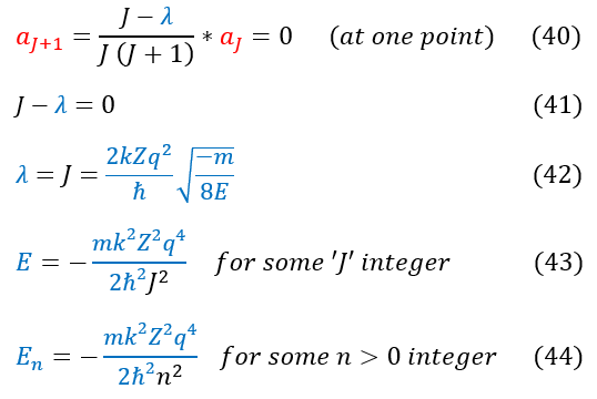
40: Equation 32 (relationship between 'a' coefficients in the power series). For some J_max, 'a_j+1' must be zero
40 to 41: Simplify the expression
41 to 42: Solve for 'lambda' and plug in our initial expression for 'labmda' (top of page)
42 to 43: Solve for the energy 'E'
43 to 44: Equation commonly seen with 'n' (same as 'J': an index). Energy cannot be zero; 'n' must be greater than zero
NOTE: we initially stated that J (or n) started from zero. Now we know that n can actually never be zero, and the index really starts at n = 1 (we didn't know this initially, so I included the index in equations 26 - 28).We can't have 1/0.Note that the 'n' values only go up to some 'n_max.'
And that is the energy of the Hydrogen atom. There are two very important notes about this energy:
1. Bohr got this EXACT SAME result earlier by just considering the electron as a standing wave going in a circle
2. The energy of 1-electron atoms are QUANTIZED (cannot take on certain energy values; constrained by 'n')
This energy quantization mathematically arose because of the necessity for the series to converge (for the wave function to be normalized). Because not all wave functions normalize, not all energies are possible (remember, this is similar to the particle in a box situation / energy quantization).
A quick note about the Bohr model: it is wrong. Electrons do not just go in a 2D circle around the nucleus. It is crazy (lucky) that Bohr actually got the right answer. This is why the Bohr model was so famous. Before people could really comprehend this mathematically, somehow Bohr was giving them the right answers for experimental results. It had some things to do with luck, but Bohr did use quantization of angular momentum (which back then, like now, was hard for people to think about). So Bohr's model did get some things right (and was very novel to think of). Going back to the Bohr model, Bohr defined a very useful constant: the Bohr radius. We can use this constant below:
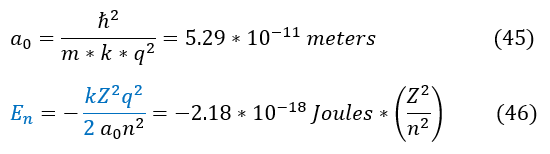
It is important to note that we can have further splitting of the energy due to spin magnetism, the zeeman effect, hyperfine splitting, and relativistic effects, but for slow moving 1-electron atoms not in a magnetic field, this is the energy.
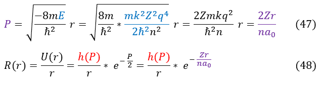
The last thing to do is to finish solving the wave function of the 1-electron atom. To begin, let us plug back in our initial definitions from the top of the page:
The last thing to do is to finish solving the wave function of the 1-electron atom. To begin, let us plug back in our initial definitions from the top of the page:
And that is the brute force way of solving the 1-electron radial equation for some 'n' index (first excited state, second excited state; we know that 'n' index's energy states as 'n' is related proportional to energy). To be clear, we start the index not at n = 0, but at n = 1. We initially started counting at J (which is the same as n) = 0, but when we solved the system, we found that energy is proportional to 1/n^2 (and hence, n can NEVER be zero).
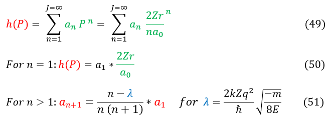
We can now solve the 1-electron system. All we need to know is h(P), which requires one initial value: a_1. Once we know a_1, we can solve for any a_n value using equation 32. We can solve for n = 1 (the ground state) below:
We can now solve the 1-electron system. All we need to know is h(P), which requires one initial value: a_1. Once we know a_1, we can solve for any a_n value using equation 32. We can solve for n = 1 (the ground state) below:
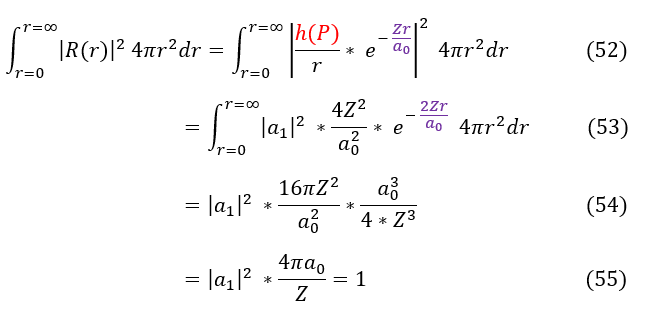
We can now normalize the ground state (integrating over 4 pi r^2 spherical shells as the L = 0 S-orbital is spherically symmetric over the integral):
In order to make sure everyone is following, let us review some key steps below:
52: The definition of normalization over all space with our function plugged in
52 to 53: Square the function
53 to 54: Take the integral
54 to 55: Simplify the integral and set the normalization to 1
Altogether, our ground state radial function for some Z effective charge of the nucleus is therefore:

|
|
|
