Without question, one of the most beautiful aspects about physics is its symmetry. There is so much symmetry, in fact, that we give it its own operator: the parity operator. Remember, operators are mathematical definitions, with no physical motivation. We only use operators to tell us information about the real world. Therefore, let us define our parity operator first, and understand its physical significance later (on this page). We will define the parity operator as so:
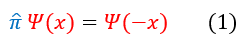
To be clear, all that the parity operator (pi) does is flip the sign of x (for higher dimensions, the parity operator will still only flips the sign of one variable). The parity operator is a function that takes in 'x' and transforms it to '-x' (gives every 'x' a minus sign). As we previously discussed, operators output significant eigenvalues by scaling a function (since its not a physically observed process, we need to mathematically differentiate the outputted value, the eigenvalue, from the initial function. This is how we do that). We have not yet found its eigenfunctions in equation 1, just its property.
One might notice that this operator has some relation to even and odd functions. To see the connection clearly, let us recall the definitions of even and odd functions below:
One might notice that this operator has some relation to even and odd functions. To see the connection clearly, let us recall the definitions of even and odd functions below:
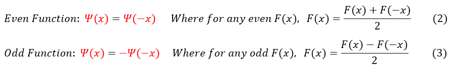
By analyzing the even and odd function definitions, we can see that if the parity operator does scale a function (is applied to its eigenfunction) by +/- 1 then the function is either even (+) or odd (-) respectively. We can explicitly say this below:
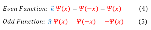
Therefore, the physical significance of the parity operator is to determine if the function is even or odd. If the function is even, the parity operator will scale the function by '1' (have an eigenvalue of '1'), and if the function is odd then the parity operator will scale the function by '-1' (have an eigenvalue of '-1').
This is useful because many wave functions we find for particles are even / odd functions (which is odd because most functions are neither even or odd). In fact, all wave functions in a symmetric (ie. even) potential in 1-dimension can be written as either even or odd ... Lets back up this statement with some math.
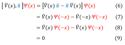
A symmetric potential, which for our case (in 1-dimension) just means an even potential, is a potential where V(x) = V(-x). Using only this definition, and our 1-dimensional (time - independent) Schrödinger equation, we can show that:
This is useful because many wave functions we find for particles are even / odd functions (which is odd because most functions are neither even or odd). In fact, all wave functions in a symmetric (ie. even) potential in 1-dimension can be written as either even or odd ... Lets back up this statement with some math.
A symmetric potential, which for our case (in 1-dimension) just means an even potential, is a potential where V(x) = V(-x). Using only this definition, and our 1-dimensional (time - independent) Schrödinger equation, we can show that:
|
|
In order to make sure everyone is following, let us review some key steps below:
6: The definition of the commutator between the potential V(x) and the parity operator
6 to 7: Distribute the parity operator to transform all 'x' to '-x'
7 to 8: It is given that V(x) is an even function, so V(x) = V(-x)
8 to 9: Simplify the expression to zero
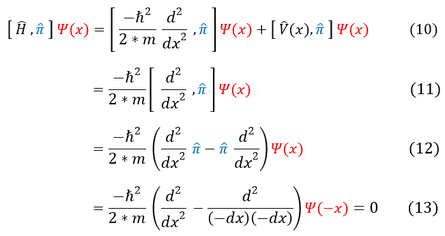
We have shown that the parity operator commutes with an even potential. We then try and commute the parity operator and the Hamiltonian in equation 10.
10 to 11: We have already shown that the potential and the parity operator commute, so we cross out that term
11 to 12: We expand the remaining commutator
12 to 13: As we flip all the signs of 'x,' we notice that the second derivative gets flips twice (the negative sign cancels)
Therefore, for an even potential, we find that the Hamiltonian does indeed commute with the parity operator.
As we previously learned (under the Introduction to Commutators page), when two operators commute then they always share a set of common eigenfunctions. While they may not share all of them, we can always find a common set. So if we find the eigenfunctions of the parity operator, we also find some of the eigenfunctions of the Hamiltonian.
We call eigenfunctions the equations which, when acted on by an operator, is uniformly scaled at every point by some constant (which we call an eigenvalue). For this problem, we will call the eigenvalue, the constant, 'c.' We can set up this problem for the parity operator below:
6: The definition of the commutator between the potential V(x) and the parity operator
6 to 7: Distribute the parity operator to transform all 'x' to '-x'
7 to 8: It is given that V(x) is an even function, so V(x) = V(-x)
8 to 9: Simplify the expression to zero
We have shown that the parity operator commutes with an even potential. We then try and commute the parity operator and the Hamiltonian in equation 10.
10 to 11: We have already shown that the potential and the parity operator commute, so we cross out that term
11 to 12: We expand the remaining commutator
12 to 13: As we flip all the signs of 'x,' we notice that the second derivative gets flips twice (the negative sign cancels)
Therefore, for an even potential, we find that the Hamiltonian does indeed commute with the parity operator.
As we previously learned (under the Introduction to Commutators page), when two operators commute then they always share a set of common eigenfunctions. While they may not share all of them, we can always find a common set. So if we find the eigenfunctions of the parity operator, we also find some of the eigenfunctions of the Hamiltonian.
We call eigenfunctions the equations which, when acted on by an operator, is uniformly scaled at every point by some constant (which we call an eigenvalue). For this problem, we will call the eigenvalue, the constant, 'c.' We can set up this problem for the parity operator below:
|
|
In order to make sure everyone is following, let us review some key steps below:
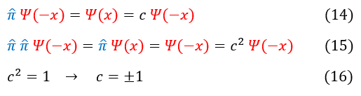
14: We apply the parity operator once to psi(-x). If psi is a wave function of the parity operator, psi(-x) is scaled by 'c'
15: We apply the parity operator twice to psi(-x). If psi is a wave function of the parity operator, psi(-x) is scaled by 'c^2'
15 to 16: Taking the last two expressions of equation 15, we see that c^2 * psi(-x) = psi(-x); hence, c^2 = 1
We find that the eigenvalue of the parity operator, in one dimension, is +/- 1. We explicitly write this out on the right.
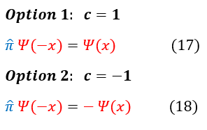
We found that:
Equation 17, which has an eigenvalue of +1, is what we previously defined as an even function.
Equation 18, which has an eigenvalue of -1, is what we previously defined as an odd function.
Hence, the parity operator's eigenfunctions, in one dimension, are only even and odd functions. Now, we know that for an even potential, the Hamiltonian must share SOME of these eigenfunctions (since they commute), but we have yet to prove that it must only share these even and odd states. To prove this fact, let us examine a simple case below:
14: We apply the parity operator once to psi(-x). If psi is a wave function of the parity operator, psi(-x) is scaled by 'c'
15: We apply the parity operator twice to psi(-x). If psi is a wave function of the parity operator, psi(-x) is scaled by 'c^2'
15 to 16: Taking the last two expressions of equation 15, we see that c^2 * psi(-x) = psi(-x); hence, c^2 = 1
We find that the eigenvalue of the parity operator, in one dimension, is +/- 1. We explicitly write this out on the right.
We found that:
Equation 17, which has an eigenvalue of +1, is what we previously defined as an even function.
Equation 18, which has an eigenvalue of -1, is what we previously defined as an odd function.
Hence, the parity operator's eigenfunctions, in one dimension, are only even and odd functions. Now, we know that for an even potential, the Hamiltonian must share SOME of these eigenfunctions (since they commute), but we have yet to prove that it must only share these even and odd states. To prove this fact, let us examine a simple case below:
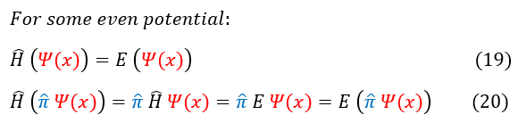
We start with equation 19: the general time - independent Schrödinger equation, where the Hamiltonian on the wave function scales the wave function by the total energy. In equation 20, we apply the same Hamiltonian to a new function: the parity operator on the wave function. We know that this new function is an even or odd wave function (as those are the only two eigenfunctions of the parity operator. For even potentials, the Hamiltonian commutes with the parity operator and we can switch their order. Now we have the Hamiltonian acting on the wave function, which we already defined in equation 19. Once we pull out the scalar, we see that the final result is just the same new function (the parity operator on the wave function) scaled by the same exact energy E. This means that the new function is indeed an eigenfunction of the Hamiltonian, with the same exact energy value as the old function.
Except, we just proved on the last page that we CANNOT have a degenerate state in 1-dimension. All degenerate states are just scalar multiples of each other, and hence, when normalized, are exactly the same. This means that, in 1-dimension for even potentials, ALL of the parity operator's eigenfunctions (the even and odd states) are indeed eigenfunctions of the Hamiltonian. We can build a complete set of basis functions, in 1-dimension for an even potential, by just using even and odd functions. The Hamiltonian does have other eigenfunctions, but we can build a complete orthogonal basis from just even and odd functions.
To recap because this is important:
For an even potential, in one dimension, we found that the Hamiltonian commutes with the parity operator. Hence, the Hamiltonian and the parity operator share some common eigenfunctions. Moreover, since every parity operator's eigenstate is degenerate to an eigenstate of the Hamiltonian, all of the even and odd eigenfunctions of the parity operator are actually also eigenfunctions of the Hamiltonian. This provides a complete orthogonal basis to work with; hence, for an even potential in 1-dimension, we can always choose our basis set of functions to be completely even or odd. This will be shown to be an incredibly useful mathematical tool while working with the wave function in 1-dimension (even potentials are actually pretty common).
|
|
|
