|
|
|
Pre-Relativity,
Special Relativity, crudely speaking, is the study of the relative differences recorded about events witnessed between two difference frames (two different observers). To discuss such events, let us define some shorthand notation with a simple example below:
Suppose John (Person A, Reference Frame S') is on a train that moves with some velocity V. Bored, John takes out a flashlight and shines it on the ceiling. The light goes up, hits a mirror, and comes back down (Event P). Meanwhile, Sam (Person B) is outside the train. Also seemingly bored, Sam additionally watches the light bounce up and down in his own reference frame (S). This example can be illustrated in the diagram below:
Suppose John (Person A, Reference Frame S') is on a train that moves with some velocity V. Bored, John takes out a flashlight and shines it on the ceiling. The light goes up, hits a mirror, and comes back down (Event P). Meanwhile, Sam (Person B) is outside the train. Also seemingly bored, Sam additionally watches the light bounce up and down in his own reference frame (S). This example can be illustrated in the diagram below:
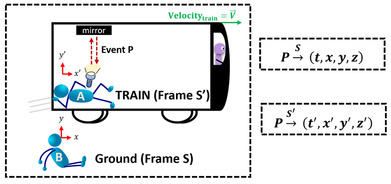
To describe this event (or any event) we need to specify which reference frame we are referring to as Sam and John will not witness the same dynamics of motion. John (person A) will watch the light bounces straight up and down only along the y axis, while Sam (Person B) will perceive the light to have some velocity in the x direction (as the train moves towards the right). Both are correct in their own frame of reference.
Unfortunately, it is tedious to keep writing out a sentence to fully define every event in everyone's frame; hence, we will switch to using 4-vector notation. 4-vectors are only matrices with 4 components, but the two main ones for relativity will be for space-time and mass-energy shown below:
Unfortunately, it is tedious to keep writing out a sentence to fully define every event in everyone's frame; hence, we will switch to using 4-vector notation. 4-vectors are only matrices with 4 components, but the two main ones for relativity will be for space-time and mass-energy shown below:
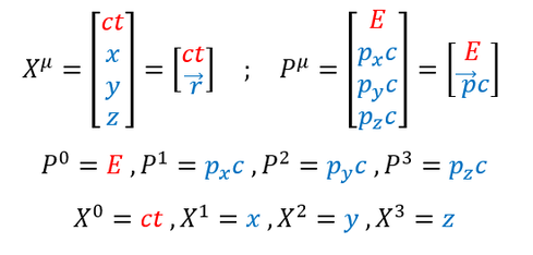
The mu above the X and P tell us that it is a 4-vector (not just any vector with any components). Note that sometimes you will see a J instead if you are only looking at the 3 spacial components.
4-Vectors can be a bit tricky as there are two main types: covariance (mu in subscript) and contravariance (mu in superscript). To be honest, the definitions are a bit confusing (and completely irrelevant to the average physicist), but they can be defined as shown below:
1. Covariant Vectors: Are perpendicular projections from the axes. Note, in a 2D world, if a coordinate system had non-perpendicular axes (non-orthogonal basis functions), then these perpendicular projections will not accurately represent the second axis/basis (this is circular logic I know). What this means however is that the covariant form (perpendicular projection) of an image's coordinates cannot be directly scaled to additionally scale the image (inverse logic needed). Common examples are gradients (or most functions with a 1/unit).
2. Contravariant Vectors: Are the opposite of Covariant vectors in that they produce parallel projections to the axes. Therefore, if your scale an image's Contravariant vector, then you are actually just scaling the axes itself (as your contravariant projection will always produce the other axis). This will therefore directly scale the image's coordinates and the image itself. Common examples are distance, time, and velocity.
Now, if those definitions confuse you, don't worry too much about it. While it is good to know, it really does not matter for relativity (In fact, I add it only to be rigorous). What is important is how we mathematically deal with 4-vectors. 4-vectors follow the standard rules for addition and subtraction, but we can define their dot product below:
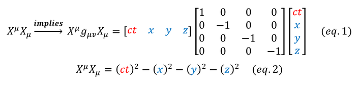
Equation 1: Notice that we seemingly add the 4x4 g-term arbitrarily. It actually has to do with preserving the invariance in Minkowski space (to be discussed much later). For now, just note that anytime someone uses this operation, they do NOT mean regular dot product (not mathematically or physically).
Additionally, note that some physicists like to take the negative expression of what I wrote in equation 2 above (using an eta term instead of the g term where eta = - g). This is completely arbitrary as invariance does not depend on the sign of the equation and hence the reasoning (which we will discuss at length later) will be the same.
Additionally, note that some physicists like to take the negative expression of what I wrote in equation 2 above (using an eta term instead of the g term where eta = - g). This is completely arbitrary as invariance does not depend on the sign of the equation and hence the reasoning (which we will discuss at length later) will be the same.
|
|
|
